Naive Bayes
استكشف Naive Bayes، وهي خوارزمية تعلم آلي رئيسية للتصنيف. تعرف على فرضية الاستقلالية الخاصة بها، وتطبيقاتها في معالجة اللغات الطبيعية، وكيفية مقارنتها بـ Ultralytics YOLO26.
سذاجة بايز (Naive Bayes) هي عائلة من الخوارزميات الاحتمالية المستخدمة على نطاق واسع في تعلم الآلة لمهام التصنيف. استناداً إلى المبادئ الإحصائية، تطبق هذه الخوارزمية مبرهنة بايز مع افتراض استقلالية قوي (أو "ساذج") بين الميزات. على الرغم من بساطتها، تعد هذه الطريقة فعالة للغاية لتصنيف البيانات، خاصة في السيناريوهات التي تتضمن مجموعات بيانات عالية الأبعاد مثل النصوص. وهي بمثابة حجر أساس في مجال التعلم الخاضع للإشراف، حيث توفر توازناً بين الكفاءة الحسابية والأداء التنبئي.
Link to this sectionالمفهوم الأساسي: الافتراض "الساذج"#
تتنبأ الخوارزمية باحتمالية انتمائية نقطة بيانات معينة إلى فئة محددة. ينبع الجانب "الساذج" من الافتراض بأن وجود ميزة معينة في فئة ما لا علاقة له بوجود أي ميزة أخرى. على سبيل المثال، قد تُعتبر الفاكهة تفاحة إذا كانت حمراء ومستديرة وقطرها حوالي 3 بوصات. يأخذ مصنف سذاجة بايز (Naive Bayes) كل نقطة من نقاط استخراج الميزات هذه بعين الاعتبار بشكل مستقل لحساب احتمالية كون الفاكهة تفاحة، بغض النظر عن أي ارتباطات محتملة بين اللون والاستدارة والحجم.
يقلل هذا التبسيط بشكل كبير من القدرة الحسابية المطلوبة لـ تدريب النموذج، مما يجعل الخوارزمية سريعة بشكل استثنائي. ومع ذلك، نظراً لأن بيانات العالم الحقيقي غالباً ما تحتوي على متغيرات تابعة وعلاقات معقدة، فقد يحد هذا الافتراض أحياناً من أداء النموذج مقارنة بالبنيات الأكثر تعقيداً.
Link to this sectionتطبيقات العالم الحقيقي#
تتألق خوارزمية سذاجة بايز (Naive Bayes) في التطبيقات التي تكون فيها السرعة أمراً بالغ الأهمية ويكون افتراض الاستقلالية مقبولاً إلى حد معقول.
- تصفية البريد المزعج (Spam): أحد أشهر استخدامات سذاجة بايز (Naive Bayes) هو في معالجة اللغات الطبيعية (NLP) لتصفية البريد الإلكتروني. يحلل المصنف تكرار الكلمات (الرموز) في البريد الإلكتروني لتحديد ما إذا كان "مزعجاً" (Spam) أو "مشروعاً" (Ham). ويحسب احتمالية كون الرسالة مزعجة بالنظر إلى وجود كلمات مثل "مجاني" أو "فائز" أو "عاجل". يعتمد هذا التطبيق بشكل كبير على تقنيات تصنيف النصوص للحفاظ على نظافة صناديق البريد.
- تحليل المشاعر: تستخدم الشركات هذه الخوارزمية لقياس الرأي العام من خلال تحليل مراجعات العملاء أو منشورات وسائل التواصل الاجتماعي. من خلال ربط كلمات معينة بمشاعر إيجابية أو سلبية، يمكن للنموذج تصنيف كميات هائلة من الملاحظات بسرعة. وهذا يسمح للشركات بإجراء تحليل مشاعر واسع النطاق لفهم تصور العلامة التجارية دون قراءة كل تعليق يدوياً.
Link to this sectionمقارنة بين سذاجة بايز (Naive Bayes) والتعلم العميق في رؤية الحاسوب#
بينما تعد سذاجة بايز (Naive Bayes) قوية للنصوص، إلا أنها غالباً ما تواجه صعوبات في المهام الإدراكية مثل رؤية الحاسوب (CV). في الصورة، تكون قيمة البكسل الواحد عادةً معتمدة بشكل كبير على جيرانه (على سبيل المثال، مجموعة من البكسلات التي تشكل حافة أو ملمساً). ينهار افتراض الاستقلالية هنا.
بالنسبة للمهام البصرية المعقدة مثل اكتشاف الكائنات، يفضل استخدام نماذج التعلم العميق (DL) الحديثة. تستخدم بنيات مثل YOLO26 طبقات تلافيفية لالتقاط التسلسلات الهرمية المكانية وتفاعلات الميزات التي تتجاهلها سذاجة بايز (Naive Bayes). وفي حين توفر سذاجة بايز (Naive Bayes) أساساً احتماليًا، فإن نماذج مثل YOLO26 توفر الدقة العالية المطلوبة للقيادة الذاتية أو التشخيص الطبي. ولإدارة مجموعات البيانات المطلوبة لنماذج الرؤية المعقدة هذه، توفر أدوات مثل منصة Ultralytics سير عمل مبسطاً للتعليق والتدريب يتجاوز بكثير مجرد التعامل مع البيانات الجدولية البسيطة.
Link to this sectionمقارنة مع الشبكات البايزية#
من المفيد تمييز سذاجة بايز (Naive Bayes) عن المفهوم الأوسع لـ الشبكة البايزية.
- سذاجة بايز (Naive Bayes): شكل متخصص ومبسط من الشبكة البايزية حيث تشير جميع عقد التنبؤ مباشرة إلى عقدة الفئة، ولا توجد اتصالات بين المتنبئات.
- الشبكات البايزية: تستخدم هذه الشبكات رسماً بيانياً موجهاً بلا دورات (DAG) لنمذجة التبعيات الشرطية المعقدة بين المتغيرات. يمكنها تمثيل علاقات سببية يبسطها النهج "الساذج".
Link to this sectionمثال على التنفيذ#
بينما تركز حزمة ultralytics على التعلم العميق، عادةً ما يتم تنفيذ سذاجة بايز (Naive Bayes) باستخدام مكتبة scikit-learn القياسية. يوضح المثال التالي كيفية تدريب نموذج سذاجة بايز الغاوسي (Gaussian Naive Bayes)، وهو مفيد للبيانات المستمرة.
import numpy as np
from sklearn.naive_bayes import GaussianNB

# Sample training data: [height (cm), weight (kg)] and Labels (0: Cat A, 1: Cat B)
X = np.array([[175, 70], [180, 80], [160, 50], [155, 45]])
y = np.array([0, 0, 1, 1])

# Initialize and train the classifier
model = GaussianNB()
model.fit(X, y)

# Predict class for a new individual [172 cm, 75 kg]
# Returns the predicted class label (0 or 1)
print(f"Predicted Class: {model.predict([[172, 75]])[0]}")
Link to this sectionالمزايا والقيود#
تتمثل الميزة الرئيسية لسذاجة بايز (Naive Bayes) في انخفاض زمن الاستدلال بشكل كبير ومتطلبات الأجهزة الدنيا. يمكنها تفسير مجموعات بيانات ضخمة قد تبطئ خوارزميات أخرى مثل آلات ناقل الدعم (SVM). علاوة على ذلك، فهي تؤدي أداءً جيداً بشكل مدهش حتى عندما يتم انتهاك افتراض الاستقلالية.
ومع ذلك، فإن اعتمادها على الميزات المستقلة يعني أنها لا تستطيع التقاط التفاعلات بين السمات. إذا كان التنبؤ يعتمد على مزيج من الكلمات (مثل "ليس جيداً")، فقد تواجه سذاجة بايز (Naive Bayes) صعوبات مقارنة بالنماذج التي تستخدم آليات الانتباه أو المحولات (Transformers). بالإضافة إلى ذلك، إذا لم تكن الفئة الموجودة في بيانات الاختبار موجودة في مجموعة التدريب، فإن النموذج يعين لها احتمالية صفرية، وهي مشكلة غالباً ما يتم حلها بـ تنعيم لابلاس.