Kalman Filter (KF)
Explore how the Kalman Filter estimates system states under uncertainty. Learn to use it for object tracking with Ultralytics YOLO26 to improve AI precision.
A Kalman Filter (KF) is a recursive mathematical algorithm used to estimate the state of a dynamic system over time. Originally introduced by Rudolf E. Kálmán, this technique is essential for processing data that is uncertain, inaccurate, or contains random variations, often referred to as "noise." By combining a series of measurements observed over time containing statistical inaccuracies, the Kalman Filter produces estimates of unknown variables that are more precise than those based on a single measurement alone. In the fields of machine learning (ML) and artificial intelligence (AI), it acts as a critical tool for predictive modeling, smoothing out jagged data points to reveal the true underlying trend.
Link to this sectionHow the Kalman Filter Works#
The algorithm operates on a two-step cycle: prediction and update (also known as correction). It assumes that the underlying system is linear and that the noise follows a Gaussian distribution (bell curve).
-
Prediction: The filter uses a physical model to project the current state forward in time. For example, if an object is moving at a constant velocity, the filter predicts its next position based on standard kinematic equations. This step also estimates the uncertainty associated with that prediction.
-
Update: When a new measurement arrives from a sensor, the filter compares the predicted state with the observed data. It calculates a weighted average—determined by the Kalman Gain—which places more trust in the value (prediction or measurement) that has less uncertainty. The result is a refined state estimation that serves as the baseline for the next cycle.
Link to this sectionApplications in Computer Vision and AI#
While originally rooted in control theory and aerospace navigation, the Kalman Filter is now ubiquitous in modern computer vision (CV) pipelines.
- Object Tracking: This is the most common use case. When a detection model like YOLO26 identifies an object in a video frame, it provides a static snapshot. To understand movement, trackers like BoT-SORT utilize Kalman Filters to link detections across frames. If an object is temporarily occluded (blocked from view), the filter uses the object's previous velocity to predict its location, preventing the system from losing the "track" or switching IDs.
- Sensor Fusion in Robotics: In robotics, machines must navigate using multiple noisy sensors. A delivery robot might use GPS (which can drift), wheel encoders (which can slip), and IMUs (which are noisy). The Kalman Filter fuses these disparate inputs to provide a single, reliable coordinate for navigation, essential for safe autonomous vehicles operations.
Link to this sectionDistinguishing Related Concepts#
It is helpful to differentiate the standard Kalman Filter from its variations and alternatives found in statistical AI:
- Kalman Filter vs. Extended Kalman Filter (EKF): The standard KF assumes the system follows linear equations (straight lines). However, real-world motion—like a drone banking a turn—is often non-linear. The EKF solves this by linearizing the system dynamics at each step using derivatives, making it suitable for complex trajectories.
- Kalman Filter vs. Particle Filter: While KFs rely on Gaussian assumptions, particle filters use a set of random samples (particles) to represent probability distributions. Particle filters are more flexible for non-Gaussian noise but require significantly more computational power, potentially affecting real-time inference speeds.
Link to this sectionImplementation Example#
In the Ultralytics ecosystem, Kalman Filters are integrated directly into tracking algorithms. You do not need to write the equations manually; you can leverage them by enabling tracking modes. The Ultralytics Platform allows you to manage datasets and train models that can be easily deployed with these tracking capabilities.
Here is a concise example using Python to perform tracking with YOLO26, where the underlying tracker automatically applies Kalman filtering to smooth the bounding box movements:
from ultralytics import YOLO

# Load the latest YOLO26 model
model = YOLO("yolo26n.pt")

# Run tracking on a video source
# The 'botsort' tracker uses Kalman Filters internally for state estimation
results = model.track(source="traffic_video.mp4", tracker="botsort.yaml")

# Process results
for result in results:
    # Access the tracked IDs (assigned and maintained via KF logic)
    if result.boxes.id is not None:
        print(f"Tracked IDs in frame: {result.boxes.id.cpu().numpy()}")
Link to this sectionImportance for Data Quality#
In real-world deployment, data is rarely perfect. Cameras suffer from motion blur, and sensors experience signal noise. The Kalman Filter acts as a sophisticated data cleaning mechanism within the decision loop. By continuously refining estimates, it ensures that AI agents operate based on the most probable reality rather than reacting to every momentary glitch in the input stream. This reliability is paramount for safety-critical applications, from monitoring airport operations to precise industrial automation.