Long Short-Term Memory (LSTM)

Long short-term memory (LSTM) is a recurrent neural network (RNN) architecture that adds a gated memory, the cell state, alongside the hidden state of a simple RNN, so it can carry information across hundreds or thousands of time steps. Sepp Hochreiter and Jürgen Schmidhuber introduced it in 1997 to overcome the vanishing gradient problem that keeps simple RNNs from learning long-range dependencies, and their paper reported bridging time lags of more than 1,000 steps. In the 2010s, LSTMs powered speech recognition, machine translation, and handwriting recognition, until transformers took over most language tasks. They remain common for time series analysis, sensor streams, and on-device models, where a constant-size state and a constant cost per step matter.

How an LSTM Cell Works#

At each time step t, an LSTM reads the input xₜ and the previous hidden state hₜ₋₁ and computes three gates and a candidate, each with its own weights. The gates use the sigmoid function, so every element lies between 0 and 1, and the candidate uses tanh, so it lies between −1 and 1:

• Forget gate: fₜ = σ(W_f xₜ + U_f hₜ₋₁ + b_f) decides how much of each element of the old cell state to keep.
• Input gate: iₜ = σ(W_i xₜ + U_i hₜ₋₁ + b_i) decides how much of the candidate to write.
• Candidate: gₜ = tanh(W_g xₜ + U_g hₜ₋₁ + b_g) proposes new content.
• Output gate: oₜ = σ(W_o xₜ + U_o hₜ₋₁ + b_o) decides how much of the cell to expose.

The two states then update as cₜ = fₜ ⊙ cₜ₋₁ + iₜ ⊙ gₜ and hₜ = oₜ ⊙ tanh(cₜ), where ⊙ is element-wise multiplication. The cell state is the long-term memory, and the hidden state is the short-term output that feeds the next layer and the next step.

The cell update is additive. The gradient of cₜ with respect to cₜ₋₁ is fₜ, element by element, so when the forget gate stays near 1 the error signal passes back through many steps almost unchanged, the path the original paper called the constant error carousel. The 1997 LSTM had no forget gate, and its cells could only accumulate. Felix Gers, Schmidhuber, and Fred Cummins added the forget gate in 2000 so cells could reset, and every standard LSTM has one today. Initializing the forget-gate bias to 1, which Rafal Jozefowicz and colleagues recommended in 2015, keeps the gate open early in training so the network starts out remembering.

LSTM in PyTorch#

PyTorch's nn.LSTM runs the cell over a whole sequence and returns the hidden state at every step plus the final hidden and cell states. The snippet below classifies short video clips from per-frame feature vectors, such as those a convolutional neural network (CNN) extracts from each frame:

import torch
from torch import nn

# 8 video clips, 16 frames each, 512 features per frame: (batch, time, features)
clips = torch.randn(8, 16, 512)

# One LSTM layer with a 128-dim hidden state, and a classifier over 5 actions
lstm = nn.LSTM(input_size=512, hidden_size=128, batch_first=True)
classifier = nn.Linear(128, 5)

# output holds h at every step; h_n and c_n are the final hidden and cell states
output, (h_n, c_n) = lstm(clips)
logits = classifier(h_n[-1])
print(f"output {tuple(output.shape)}, h_n {tuple(h_n.shape)}, c_n {tuple(c_n.shape)}, logits {tuple(logits.shape)}")

# Each weight matrix stacks four blocks of 128 rows: input gate, forget gate, candidate, output gate
print(f"Input weights {tuple(lstm.weight_ih_l0.shape)}, recurrent weights {tuple(lstm.weight_hh_l0.shape)}")

It prints output (8, 16, 128), h_n (1, 8, 128), c_n (1, 8, 128), logits (8, 5) and Input weights (512, 512), recurrent weights (512, 128). The final hidden state summarizes each 16-frame clip for the five-way classifier, and each weight matrix has 4 × 128 = 512 rows because PyTorch stores the four gate blocks in one matrix.

LSTM vs. Related Architectures#

• Simple RNN: Rewrites its whole state through one tanh layer at every step, so gradients shrink or grow geometrically with sequence length and long-range dependencies are hard to learn.
• GRU: Merges the cell and hidden states and uses two gates instead of three, giving three weight blocks instead of four and three quarters of the LSTM's parameters at the same width. Neither wins consistently across tasks.
• Transformer: Processes all positions in parallel with self-attention, which trains far faster on GPUs and reaches distant context directly, so transformers replaced LSTMs in language modeling and translation. Attention's cost grows with context length, and an LSTM spends the same compute and memory on every new step.
• xLSTM: xLSTM, from Hochreiter's group in 2024, adds exponential gating and a matrix memory that trains in parallel. Its 7-billion-parameter language model, xLSTM 7B, was published at ICML 2025 with performance comparable to transformer models of similar size and faster inference.

Applications#

• Speech recognition: Google moved voice search to LSTM acoustic models trained with connectionist temporal classification (CTC) in 2015, and on-device recognizers long relied on stacked LSTMs.
• Machine translation: Google Neural Machine Translation, launched in 2016, stacked eight LSTM layers in its encoder and eight in its decoder.
• Flood forecasting: Google's flood forecasting system, described in Nature in 2024, uses LSTM networks to predict river flow from weather data and forecasts extreme floods in ungauged watersheds up to five days ahead.
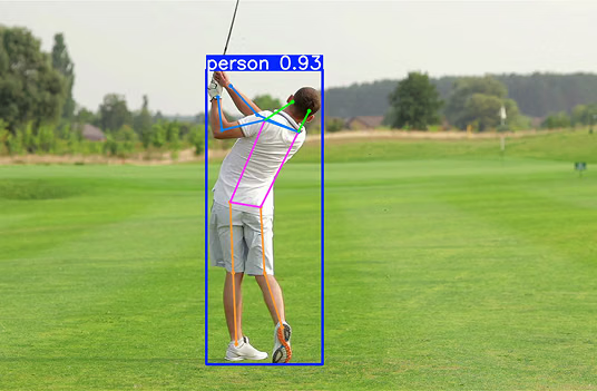
• Action recognition: A CNN encodes each video frame and an LSTM reads the sequence of frame features to label the clip, the structure the snippet above follows.
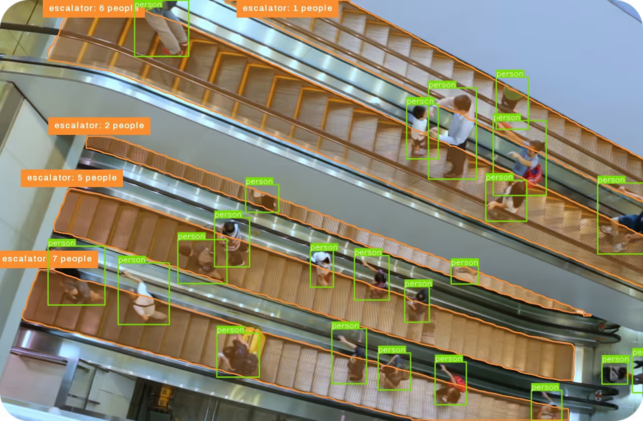
• Trajectory prediction: Social LSTM runs one LSTM per pedestrian and pools the hidden states of nearby people to forecast paths through crowds. YOLO26 in track mode assigns each person a persistent ID across video frames, which turns per-frame detections into the position histories such a forecaster reads.