Gated Recurrent Unit (GRU)

A gated recurrent unit (GRU) is a recurrent neural network (RNN) cell that processes a sequence one step at a time and uses two learned gates, an update gate and a reset gate, to decide how much of its memory to keep and how much to overwrite at each step. Kyunghyun Cho and colleagues introduced it in 2014 in an RNN encoder-decoder for machine translation. The gates let gradients flow across many time steps, so a GRU learns longer-range dependencies than a simple RNN, which suffers from the vanishing gradient problem. The GRU is a simplified relative of the long short-term memory (LSTM) network, with one hidden state instead of two and three weight blocks instead of four, and it is used for time series analysis, speech, and other sequential data.

How a GRU Works#

At each time step t, a GRU combines the current input xₜ with its previous hidden state hₜ₋₁. Two gates use the sigmoid function to output values between 0 and 1 for every element of the state:

• Reset gate: rₜ = σ(Wᵣxₜ + Uᵣhₜ₋₁ + bᵣ) decides how much of the previous state to use when proposing new content. Values near 0 let the cell ignore its history, which helps at boundaries such as the start of a new phrase.
• Update gate: zₜ = σ(W_z xₜ + U_z hₜ₋₁ + b_z) decides how much of the previous state to keep. Values near 1 copy the old state forward almost unchanged, which is how information survives over long spans.
• Candidate state: h̃ₜ = tanh(Wxₜ + U(rₜ ⊙ hₜ₋₁) + b) proposes new content from the input and the reset-scaled history, using tanh to keep values between −1 and 1.
• New state: hₜ = (1 − zₜ) ⊙ h̃ₜ + zₜ ⊙ hₜ₋₁ blends the candidate with the old state, element by element.

When the update gate stays near 1, the new state is almost a copy of the old one, and the gradient passes back through that copy with little decay. This additive path plays the same role as the cell state in an LSTM. The equations above follow the original paper, where zₜ weights the old state; some texts swap the roles of zₜ and 1 − zₜ, which describes the same cell. PyTorch's nn.GRU uses the same blend but applies the reset gate after the matrix multiplication, as rₜ ⊙ (Uhₜ₋₁ + b), a widely used variant of the candidate state.

GRU in PyTorch#

The snippet below runs a GRU over a sequence of feature vectors, such as per-frame features from a video, and compares its size with an LSTM of the same width:

import torch
from torch import nn

# A sequence of 64-dim features from 5 video frames: (batch, time, features)
frames = torch.randn(1, 5, 64)

# A GRU with a 128-dim hidden state, and an LSTM of the same size for comparison
gru = nn.GRU(input_size=64, hidden_size=128, batch_first=True)
lstm = nn.LSTM(input_size=64, hidden_size=128, batch_first=True)

# outputs holds the hidden state at every step; h_n is the final state
outputs, h_n = gru(frames)
print(f"Outputs: {tuple(outputs.shape)}, final state: {tuple(h_n.shape)}")

# GRU weights cover 3 blocks (reset, update, candidate); LSTM weights cover 4
gru_params = sum(p.numel() for p in gru.parameters())
lstm_params = sum(p.numel() for p in lstm.parameters())
print(f"GRU: {gru_params:,} parameters, LSTM: {lstm_params:,} parameters")

It prints Outputs: (1, 5, 128), final state: (1, 1, 128) and GRU: 74,496 parameters, LSTM: 99,328 parameters. The GRU returns one 128-dimensional state per frame plus the final state, which summarizes the whole sequence for a downstream classifier, and it needs exactly three quarters of the LSTM's parameters.

GRU vs. LSTM and Transformers#

• LSTM: Keeps a separate cell state alongside the hidden state and uses three gates (input, forget, and output). The GRU merges the two states and drops the output gate, so it trains faster per step with fewer parameters. In an empirical comparison by Junyoung Chung and colleagues in 2014, GRUs matched LSTMs on polyphonic music and speech signal modeling, and in practice neither wins consistently across tasks.
• Simple RNN: Overwrites its whole state at every step with no gates, so its gradients vanish or explode over long sequences and it struggles to connect events separated by long gaps.
• Transformer: Processes all positions of a sequence in parallel with attention, which trains far faster on GPUs and handles long-range context better, so transformers replaced recurrent networks in most language tasks. A GRU keeps a constant-size state and constant cost per step no matter how long the sequence gets, which still suits streaming audio, sensor data, and small devices.

Applications#

• Optical flow: RAFT, which won the ECCV 2020 best paper award, refines its flow estimate over many iterations with a convolutional GRU, a GRU whose matrix multiplications are replaced by convolutions so its state is a feature map.
• Predictive maintenance and forecasting: GRUs read streams of vibration, temperature, or demand data and predict failures or future values, often on embedded hardware where a small model matters.
• Speech and audio: On-device audio models use GRUs because they process audio frame by frame with a small, fixed memory. The RNNoise noise suppressor runs its GRU layers in real time on an ordinary CPU.
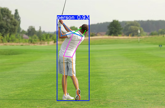
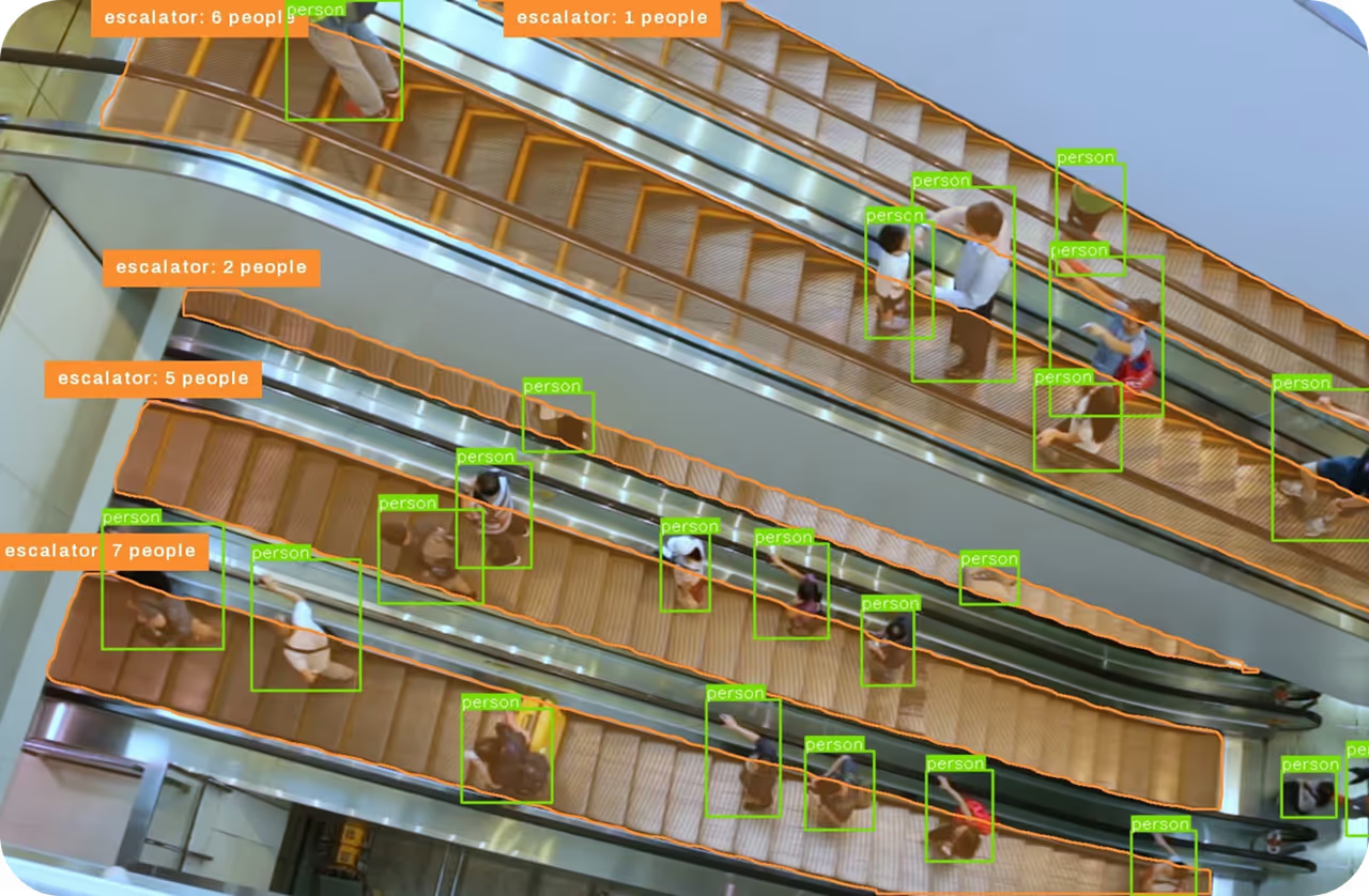
• Action recognition: A GRU reads a sequence of per-frame features or keypoints and outputs an action label for the clip. YOLO26 in track mode assigns each person a persistent ID across frames, which yields the per-person sequences of boxes or pose keypoints that such a GRU classifies.