Receptive Field
Explore how the receptive field defines what a neural network sees. Learn how Ultralytics YOLO26 optimizes spatial context to detect objects of all sizes effectively.
In the domain of computer vision (CV) and deep learning, the receptive field refers to the specific region of an input image that a particular neuron in a neural network (NN) "sees" or analyzes. Conceptually, it functions similarly to the field of view of a human eye or a camera lens. It determines how much spatial context a model can perceive at any given layer. As data progresses through a Convolutional Neural Network (CNN), the receptive field typically expands, allowing the system to transition from identifying tiny, local details—like edges or corners—to understanding complex, global structures like entire objects or scenes.
Link to this sectionThe Mechanics Of Receptive Fields#
The size and depth of the receptive field are dictated by the network's architecture. In the initial layers, neurons usually have a small receptive field, focusing on a tiny cluster of pixels to capture fine-grained textures. As the network deepens, operations such as pooling layers and strided convolutions effectively downsample the feature maps. This process allows subsequent neurons to aggregate information from a much larger portion of the original input.
Modern architectures, including the state-of-the-art Ultralytics YOLO26, are engineered to balance these fields meticulously. If the receptive field is too narrow, the model may fail to recognize large objects because it cannot perceive the entire shape. Conversely, if the field is excessively broad without maintaining resolution, the model might miss small objects. To address this, engineers often use dilated convolutions (also known as atrous convolutions) to expand the receptive field without reducing the spatial resolution, a technique vital for high-precision tasks like semantic segmentation.
Link to this sectionReal-World Applications#
Optimizing the receptive field is critical for the success of various AI solutions.
- Autonomous Driving: In AI for automotive, perception systems must simultaneously track minute details and large obstacles. A vehicle needs a small receptive field to identify distant traffic lights, while simultaneously requiring a large receptive field to understand the trajectory of a nearby truck or the curvature of the road lane. This multi-scale perception ensures better AI safety and decision-making.
- Medical Diagnostics: When applying AI in healthcare, radiologists rely on models to spot anomalies in scans. For identifying brain tumors, the network requires a large receptive field to understand the brain's overall symmetry and structure. However, to detect micro-calcifications in mammography, the model relies on early layers with small receptive fields sensitive to subtle texture changes.
Link to this sectionDistinguishing Related Concepts#
To fully understand network design, it is helpful to differentiate the receptive field from similar terms:
- Receptive Field vs. Kernel: The kernel (or filter) size defines the dimensions of the sliding window (e.g., 3x3) for a single convolution operation. The receptive field is an emergent property representing the total accumulated input area affecting a neuron. A stack of multiple 3x3 kernels will result in a receptive field much larger than 3x3.
- Receptive Field vs. Feature Map: A feature map is the output volume produced by a layer, containing the learned representations. The receptive field describes the relationship between a single point on that feature map and the original input image.
- Receptive Field vs. Context Window: While both terms refer to the scope of perceived data, "context window" is typically used in Natural Language Processing (NLP) or video analysis to denote a temporal or sequential span (e.g., token limit). Receptive field strictly refers to the spatial area in grid-like data (images).
Link to this sectionPractical Usage In Code#
State-of-the-art models like the newer YOLO26 utilize Feature Pyramid Networks (FPN) to maintain effective receptive fields for objects of all sizes. The following example shows how to load a model and perform object detection, leveraging these internal architectural optimizations automatically. Users looking to train their own models with optimized architectures can utilize the Ultralytics Platform for seamless dataset management and cloud training.
from ultralytics import YOLO

# Load the latest YOLO26 model with optimized multi-scale receptive fields
model = YOLO("yolo26n.pt")

# Run inference; the model aggregates features from various receptive field sizes
results = model("https://ultralytics.com/images/bus.jpg")

# Display the results, detecting both large (bus) and small (person) objects
results[0].show()