Optical Flow
Explora os fundamentos do fluxo ótico em visão computacional. Aprende como vetores de movimento impulsionam a compreensão de vídeo e melhoram o rastreio no Ultralytics YOLO26.
O fluxo óptico é o padrão de movimento aparente de objetos, superfícies e bordas em uma cena visual, causado pelo movimento relativo entre um observador e uma cena. No campo da visão computacional, este conceito é fundamental para a compreensão da dinâmica temporal dentro de sequências de vídeo. Ao analisar o deslocamento de pixels entre dois quadros consecutivos, os algoritmos de fluxo óptico geram um campo vetorial onde cada vetor representa a direção e a magnitude do movimento de um ponto específico. Esta pista visual de baixo nível permite que sistemas de inteligência artificial percebam não apenas o que está em uma imagem, mas como ela está se movendo, preenchendo a lacuna entre a análise de imagem estática e a compreensão de vídeo dinâmica.
Link to this sectionMecanismos Principais do Fluxo Óptico#
O cálculo do fluxo óptico geralmente depende da suposição de constância de brilho, que pressupõe que a intensidade de um pixel em um objeto permanece constante de um quadro para o próximo, mesmo enquanto ele se move. Os algoritmos utilizam este princípio para resolver vetores de movimento usando duas abordagens principais:
- Fluxo Óptico Esparso: Este método calcula o vetor de movimento para um subconjunto específico de características distintas, como cantos ou bordas, detectadas via extração de características. Algoritmos como o método de Lucas-Kanade são computacionalmente eficientes e ideais para tarefas de inferência em tempo real onde rastrear pontos específicos de interesse é suficiente.
- Fluxo Óptico Denso: Esta abordagem computa um vetor de movimento para cada pixel individual no quadro. Embora seja significativamente mais intensiva computacionalmente, ela fornece um mapa de movimento abrangente essencial para tarefas detalhadas como segmentação de imagem e análise estrutural. Arquiteturas modernas de deep learning frequentemente superam os métodos matemáticos tradicionais na estimativa de fluxo denso ao aprender padrões de movimento complexos a partir de grandes conjuntos de dados.
Link to this sectionFluxo Óptico vs. Rastreamento de Objetos#
Embora muitas vezes usados em conjunto, é vital distinguir o fluxo óptico do rastreamento de objetos. O fluxo óptico é uma operação de baixo nível que descreve o movimento instantâneo dos pixels; ele não compreende inerentemente a identidade ou a persistência do objeto.
Em contraste, o rastreamento de objetos é uma tarefa de alto nível que localiza entidades específicas e atribui a elas um ID consistente ao longo do tempo. Rastreadores avançados, como aqueles integrados ao Ultralytics YOLO26, normalmente realizam detecção de objetos para encontrar o objeto e, em seguida, usam pistas de movimento — às vezes derivadas do fluxo óptico — para associar detecções entre quadros. O fluxo óptico responde "quão rápido estes pixels estão se movendo agora", enquanto o rastreamento responde "para onde foi o Carro nº 5?"
Link to this sectionAplicações no Mundo Real#
A capacidade de estimar o movimento ao nível do pixel impulsiona uma ampla gama de tecnologias sofisticadas:
- Veículos Autônomos e Robótica: O fluxo óptico é usado para odometria visual, permitindo que um robô ou carro estime seu próprio movimento em relação ao ambiente. Ele também auxilia na estimativa de profundidade e na prevenção de obstáculos ao analisar a rapidez com que os objetos no campo visual estão se expandindo ou se movendo.
- Estabilização de Vídeo: Câmeras e softwares de edição usam vetores de fluxo para detectar tremores involuntários da câmera. Ao compensar este movimento global, os sistemas podem estabilizar digitalmente a filmagem. Este é um recurso padrão em eletrônicos de consumo modernos, como smartphones e câmeras de ação.
- Reconhecimento de Ação: Em análises esportivas e segurança, a análise do fluxo temporal de pixels ajuda os sistemas a identificar ações humanas complexas. Por exemplo, modelos de estimativa de pose podem ser aumentados com dados de fluxo para distinguir entre uma pessoa caminhando ou correndo com base na velocidade do movimento dos membros.
- Compressão de Vídeo: Padrões como a codificação de vídeo MPEG dependem fortemente da estimativa de movimento. Em vez de armazenar cada quadro completo, o codec armazena o fluxo óptico (vetores de movimento) e a diferença (residual) entre os quadros, reduzindo significativamente os tamanhos de arquivo para streaming e armazenamento.
Link to this sectionExemplo de Implementação#
O exemplo a seguir demonstra como calcular o fluxo óptico denso usando a biblioteca OpenCV, uma ferramenta padrão no ecossistema de visão computacional. Este snippet usa o algoritmo Farneback para gerar um mapa de fluxo entre dois quadros consecutivos.
import cv2
import numpy as np

# Simulate two consecutive frames (replace with actual image paths)
frame1 = np.zeros((100, 100, 3), dtype=np.uint8)
frame2 = np.zeros((100, 100, 3), dtype=np.uint8)
cv2.rectangle(frame1, (20, 20), (40, 40), (255, 255, 255), -1)  # Object at pos 1
cv2.rectangle(frame2, (25, 25), (45, 45), (255, 255, 255), -1)  # Object moved

# Convert to grayscale for flow calculation
prvs = cv2.cvtColor(frame1, cv2.COLOR_BGR2GRAY)
next = cv2.cvtColor(frame2, cv2.COLOR_BGR2GRAY)

# Calculate dense optical flow
flow = cv2.calcOpticalFlowFarneback(prvs, next, None, 0.5, 3, 15, 3, 5, 1.2, 0)

# Compute magnitude and angle of 2D vectors
mag, ang = cv2.cartToPolar(flow[..., 0], flow[..., 1])

print(f"Max motion detected: {np.max(mag):.2f} pixels")
Para aplicações de alto nível que exigem persistência de objetos em vez de movimento bruto de pixels, você deve considerar os modos de rastreamento disponíveis no Ultralytics YOLO11 e no YOLO26. Estes modelos abstraem a complexidade da análise de movimento, fornecendo IDs de objetos e trajetórias robustas prontos para uso em tarefas que variam desde monitoramento de tráfego até análise de varejo.