DBSCAN (Density-Based Spatial Clustering of Applications with Noise)
Explore DBSCAN for density-based clustering and anomaly detection. Learn how it identifies arbitrary shapes and noise in datasets alongside Ultralytics YOLO26.
DBSCAN (Density-Based Spatial Clustering of Applications with Noise) is a powerful unsupervised learning algorithm used to identify distinct groups within data based on density. Unlike traditional clustering methods that assume spherical clusters or require a predetermined number of groups, DBSCAN locates regions of high density separated by areas of low density. This capability allows it to discover clusters of arbitrary shapes and sizes, making it exceptionally effective for analyzing complex real-world datasets where the underlying structure is unknown. A key advantage of this algorithm is its built-in anomaly detection, as it automatically classifies points in low-density regions as noise rather than forcing them into a cluster.
Link to this sectionCore Concepts and Parameters#
The algorithm operates by defining a neighborhood around each data point and counting how many other points fall within that vicinity. Two primary hyperparameters control this process, requiring careful hyperparameter tuning to match the specific characteristics of the data:
- Epsilon (eps): This parameter specifies the maximum radius around a point to search for neighbors. It defines the "reachability" distance.
- Minimum Points (minPts): This sets the minimum number of data points required within the Epsilon radius to form a dense region or "core."
Based on these parameters, DBSCAN categorizes every point in the dataset into one of three types:
-
Core Points: Points that have at least
minPtsneighbors within theepsradius. These points form the interior of a cluster. -
Border Points: Points that are within the
epsradius of a core point but have fewer thanminPtsneighbors themselves. These form the edges of a cluster. -
Noise Points: Points that are neither core nor border points. These are effectively treated as outliers, which is useful for tasks like outlier detection.
Link to this sectionDBSCAN vs. K-Means Clustering#
While both are fundamental to machine learning (ML), DBSCAN offers distinct advantages over K-Means Clustering in specific scenarios. K-Means relies on centroids and Euclidean distance, often assuming clusters are convex or spherical. This can lead to poor performance on elongated or crescent-shaped data. In contrast, DBSCAN's density-based approach allows it to follow the natural contours of the data distribution.
Another significant difference lies in initialization. K-Means requires the user to specify the number of clusters (k) in advance, which can be challenging without prior knowledge. DBSCAN infers the number of clusters naturally from the data density. Additionally, K-Means is sensitive to outliers because it forces every point into a group, potentially skewing the cluster centers. DBSCAN's ability to label points as noise prevents data anomalies from contaminating valid clusters, ensuring cleaner results for downstream tasks like predictive modeling.
Link to this sectionReal-World Applications#
DBSCAN is widely applied in industries requiring spatial analysis and robust noise handling.
- Geospatial Analysis: In urban planning and logistics, analysts use DBSCAN to group GPS coordinates from delivery fleets or ride-sharing services. By identifying high-density drop-off zones, companies can optimize route planning and warehouse locations. For example, AI in logistics often involves clustering delivery stops to improve efficiency.
- Vision-Based Anomaly Detection: In manufacturing, visual inspection systems powered by models like YOLO26 might detect surface defects. DBSCAN can cluster the coordinates of these defects on a product map. Isolated detections might be dismissed as sensor noise, while dense clusters indicate a systematic manufacturing flaw, triggering an alert for quality inspection.
Link to this sectionCode Example: Clustering Detection Centroids#
In computer vision workflows, developers often use the Ultralytics Platform to train object detectors and then post-process the results. The following example demonstrates how to use the sklearn library to cluster the centroids of detected objects. This helps in grouping detections that are spatially related, potentially merging multiple bounding boxes for the same object or identifying groups of objects.
import numpy as np
from sklearn.cluster import DBSCAN

# Simulated centroids of objects detected by YOLO26
# [x, y] coordinates representing object locations
centroids = np.array(
    [
        [100, 100],
        [102, 104],
        [101, 102],  # Cluster 1 (Dense group)
        [200, 200],
        [205, 202],  # Cluster 2 (Another group)
        [500, 500],  # Noise (Outlier)
    ]
)

# Initialize DBSCAN with a radius (eps) of 10 and min_samples of 2
# This groups points close to each other
clustering = DBSCAN(eps=10, min_samples=2).fit(centroids)

# Labels: 0, 1 are cluster IDs; -1 represents noise
print(f"Cluster Labels: {clustering.labels_}")
# Output: [ 0  0  0  1  1 -1]
Link to this sectionIntegration with Deep Learning#
While DBSCAN is a classic algorithm, it pairs effectively with modern deep learning. For instance, high-dimensional features extracted from a convolutional neural network (CNN) can be reduced using dimensionality reduction techniques like PCA or t-SNE before applying DBSCAN. This hybrid approach allows for clustering complex image data based on semantic similarity rather than just pixel location. This is particularly useful in unsupervised learning scenarios where labeled training data is scarce, helping researchers organize vast archives of unlabeled images efficiently.