Optical Flow
컴퓨터 비전에서 광학 흐름(Optical Flow)의 기초를 탐구해 보십시오. 모션 벡터가 비디오 이해를 어떻게 구동하고 Ultralytics YOLO26에서 추적 기능을 향상시키는지 배우십시오.
옵티컬 플로우는 관찰자와 장면 사이의 상대적인 움직임으로 인해 시각적 장면 내의 객체, 표면 및 가장자리에서 나타나는 겉보기 운동의 패턴입니다. 컴퓨터 비전 분야에서 이 개념은 비디오 시퀀스 내의 시간적 역학을 이해하는 데 핵심적입니다. 두 개의 연속된 프레임 간 픽셀의 변위를 분석함으로써, 옵티컬 플로우 알고리즘은 각 벡터가 특정 지점의 움직임 방향과 크기를 나타내는 벡터 필드를 생성합니다. 이러한 저수준 시각적 단서는 인공지능 시스템이 이미지 내의 내용뿐만 아니라 그것이 어떻게 움직이는지를 인식할 수 있게 하여, 정적 이미지 분석과 동적 비디오 이해 사이의 간극을 메워줍니다.
Link to this section옵티컬 플로우의 핵심 메커니즘#
옵티컬 플로우 계산은 일반적으로 밝기 항상성 가정에 의존합니다. 이는 객체 위 픽셀의 밝기가 움직이더라도 프레임 간에 일정하게 유지된다는 가정을 말합니다. 알고리즘은 이 원리를 활용하여 다음 두 가지 주요 접근 방식으로 운동 벡터를 구합니다:
- 희소 옵티컬 플로우(Sparse Optical Flow): 이 방법은 특징 추출을 통해 감지된 모서리나 가장자리와 같은 특정 특징 집합에 대한 운동 벡터를 계산합니다. 루카스-카나데 방법(Lucas-Kanade method)과 같은 알고리즘은 계산 효율성이 뛰어나 특정 관심 지점 추적만으로 충분한 실시간 추론 작업에 이상적입니다.
- 밀집 옵티컬 플로우(Dense Optical Flow): 이 접근 방식은 프레임 내의 모든 픽셀에 대해 운동 벡터를 계산합니다. 계산 비용은 상당히 높지만, 이미지 분할 및 구조 분석과 같은 정밀한 작업에 필수적인 포괄적인 운동 지도를 제공합니다. 현대의 딥러닝 아키텍처는 방대한 데이터셋에서 복잡한 운동 패턴을 학습함으로써 밀집 흐름 추정에서 전통적인 수학적 방식을 종종 능가합니다.
Link to this section옵티컬 플로우와 객체 추적의 비교#
옵티컬 플로우와 객체 추적은 종종 함께 사용되지만, 이 둘을 구분하는 것은 매우 중요합니다. 옵티컬 플로우는 순간적인 픽셀 움직임을 기술하는 저수준 작업이며, 객체의 정체성이나 지속성을 본질적으로 이해하지 못합니다.
반면, 객체 추적은 특정 개체를 위치시키고 시간이 지남에 따라 일관된 ID를 할당하는 고수준 작업입니다. Ultralytics YOLO26에 통합된 것과 같은 고급 추적기는 일반적으로 객체 탐지를 수행하여 객체를 찾은 다음, 때로는 옵티컬 플로우에서 파생된 움직임 단서를 사용하여 프레임 간 탐지 결과를 연결합니다. 옵티컬 플로우가 "지금 이 픽셀들이 얼마나 빨리 움직이는가?"에 답한다면, 추적은 "5번 자동차가 어디로 갔는가?"에 답합니다.
Link to this section실제 애플리케이션 사례#
픽셀 수준에서 움직임을 추정하는 능력은 광범위한 첨단 기술의 원동력이 됩니다:
- 자율주행 차량 및 로봇 공학: 옵티컬 플로우는 시각적 오도메트리(visual odometry)에 사용되어 로봇이나 자동차가 환경에 대한 자신의 움직임을 추정할 수 있게 합니다. 또한 시야 내의 객체가 얼마나 빨리 확장되거나 움직이는지를 분석하여 깊이 추정 및 장애물 회피를 지원합니다.
- 비디오 안정화: 카메라 및 편집 소프트웨어는 흐름 벡터를 사용하여 의도치 않은 카메라 흔들림을 감지합니다. 시스템은 이러한 전역적 움직임을 보정하여 디지털 방식으로 영상을 안정화할 수 있습니다. 이는 스마트폰이나 액션 카메라와 같은 현대 소비자 가전의 표준 기능입니다.
- 행동 인식(Action Recognition): 스포츠 분석 및 보안 분야에서 픽셀의 시간적 흐름을 분석하면 시스템이 복잡한 인간의 행동을 식별하는 데 도움이 됩니다. 예를 들어, 자세 추정(pose estimation) 모델에 흐름 데이터를 보강하면 팔다리 움직임의 속도를 기반으로 사람이 걷고 있는지 달리고 있는지를 구분할 수 있습니다.
- 비디오 압축: MPEG 비디오 코딩과 같은 표준은 움직임 추정에 크게 의존합니다. 코덱은 전체 프레임을 저장하는 대신, 옵티컬 플로우(운동 벡터)와 프레임 간의 차이(잔차)를 저장하여 스트리밍 및 저장 공간을 위한 파일 크기를 크게 줄입니다.
Link to this section구현 예시#
다음 예제는 컴퓨터 비전 생태계의 표준 도구인 OpenCV 라이브러리를 사용하여 밀집 옵티컬 플로우를 계산하는 방법을 보여줍니다. 이 코드 조각은 Farneback 알고리즘을 사용하여 두 개의 연속된 프레임 간의 흐름 지도를 생성합니다.
import cv2
import numpy as np

# Simulate two consecutive frames (replace with actual image paths)
frame1 = np.zeros((100, 100, 3), dtype=np.uint8)
frame2 = np.zeros((100, 100, 3), dtype=np.uint8)
cv2.rectangle(frame1, (20, 20), (40, 40), (255, 255, 255), -1)  # Object at pos 1
cv2.rectangle(frame2, (25, 25), (45, 45), (255, 255, 255), -1)  # Object moved

# Convert to grayscale for flow calculation
prvs = cv2.cvtColor(frame1, cv2.COLOR_BGR2GRAY)
next = cv2.cvtColor(frame2, cv2.COLOR_BGR2GRAY)

# Calculate dense optical flow
flow = cv2.calcOpticalFlowFarneback(prvs, next, None, 0.5, 3, 15, 3, 5, 1.2, 0)

# Compute magnitude and angle of 2D vectors
mag, ang = cv2.cartToPolar(flow[..., 0], flow[..., 1])

print(f"Max motion detected: {np.max(mag):.2f} pixels")
원시 픽셀 움직임이 아닌 객체 지속성이 필요한 고수준 애플리케이션의 경우, 사용자는 Ultralytics YOLO11 및 YOLO26에서 제공하는 추적 모드를 고려해야 합니다. 이러한 모델은 움직임 분석의 복잡성을 추상화하여 교통 모니터링부터 리테일 분석에 이르는 다양한 작업을 위해 강력한 객체 ID와 궤적을 즉시 제공합니다.