Optical Flow
Erkunde die Grundlagen des optischen Flusses in der Computer-Vision. Lerne, wie Bewegungsvektoren das Videoverständnis vorantreiben und das Tracking in Ultralytics YOLO26 verbessern.
Der optische Fluss ist das Muster der scheinbaren Bewegung von Objekten, Oberflächen und Kanten in einer visuellen Szene, das durch die Relativbewegung zwischen einem Beobachter und einer Szene entsteht. Im Bereich der Computer Vision ist dieses Konzept grundlegend für das Verständnis zeitlicher Dynamiken innerhalb von Videosequenzen. Durch die Analyse der Verschiebung von Pixeln zwischen zwei aufeinanderfolgenden Bildern erzeugen Algorithmen für den optischen Fluss ein Vektorfeld, bei dem jeder Vektor die Richtung und Stärke der Bewegung eines bestimmten Punktes darstellt. Dieser visuelle Hinweis auf niedriger Ebene ermöglicht es künstlicher Intelligenz, nicht nur wahrzunehmen, was sich in einem Bild befindet, sondern auch, wie es sich bewegt. Damit wird die Lücke zwischen statischer Bildanalyse und dynamischem Video-Verständnis geschlossen.
Link to this sectionKernmechanismen des optischen Flusses#
Die Berechnung des optischen Flusses basiert im Allgemeinen auf der Annahme der Helligkeitskonstanz, die besagt, dass die Intensität eines Pixels an einem Objekt von einem Bild zum nächsten konstant bleibt, auch wenn es sich bewegt. Algorithmen nutzen dieses Prinzip, um Bewegungsvektoren mithilfe von zwei primären Ansätzen zu berechnen:
- Sparse Optical Flow: Diese Methode berechnet den Bewegungsvektor für eine bestimmte Teilmenge markanter Merkmale, wie etwa Ecken oder Kanten, die mittels Feature-Extraktion erkannt wurden. Algorithmen wie die Lucas-Kanade-Methode sind recheneffizient und ideal für Aufgaben der Echtzeit-Inferenz, bei denen die Verfolgung spezifischer Punkte von Interesse ausreicht.
- Dense Optical Flow: Dieser Ansatz berechnet einen Bewegungsvektor für jedes einzelne Pixel im Bild. Obwohl dies deutlich rechenintensiver ist, liefert er eine umfassende Bewegungskarte, die für feingranulare Aufgaben wie Bildsegmentierung und Strukturanalysen unerlässlich ist. Moderne Deep-Learning-Architekturen übertreffen bei der Schätzung des dichten Flusses oft traditionelle mathematische Methoden, indem sie komplexe Bewegungsmuster aus großen Datensätzen erlernen.
Link to this sectionOptischer Fluss vs. Objektverfolgung#
Obwohl sie oft zusammen verwendet werden, ist es wichtig, zwischen optischem Fluss und Objektverfolgung zu unterscheiden. Der optische Fluss ist ein Vorgang auf niedriger Ebene, der eine sofortige Pixelbewegung beschreibt; er versteht von sich aus keine Objektidentität oder -persistenz.
Im Gegensatz dazu ist die Objektverfolgung eine Aufgabe auf hoher Ebene, die spezifische Entitäten lokalisiert und ihnen über die Zeit eine konsistente ID zuweist. Fortschrittliche Tracker, wie sie in Ultralytics YOLO26 integriert sind, führen typischerweise eine Objekterkennung durch, um das Objekt zu finden, und nutzen dann Bewegungshinweise – manchmal abgeleitet aus dem optischen Fluss –, um Erkennungen über Bilder hinweg zuzuordnen. Der optische Fluss beantwortet die Frage „Wie schnell bewegen sich diese Pixel gerade?“, während die Verfolgung beantwortet: „Wo ist Auto Nr. 5 hingefahren?“
Link to this sectionPraxisanwendungen#
Die Fähigkeit, Bewegungen auf Pixelebene zu schätzen, ermöglicht eine breite Palette hochentwickelter Technologien:
- Autonome Fahrzeuge und Robotik: Optischer Fluss wird für die visuelle Odometrie verwendet, wodurch ein Roboter oder ein Auto seine eigene Bewegung relativ zur Umgebung schätzen kann. Er unterstützt zudem die Tiefenschätzung und die Vermeidung von Hindernissen, indem er analysiert, wie schnell sich Objekte im Sichtfeld ausdehnen oder bewegen.
- Videostabilisierung: Kameras und Bearbeitungssoftware verwenden Flussvektoren, um unbeabsichtigtes Kamerawackeln zu erkennen. Durch den Ausgleich dieser globalen Bewegung können Systeme Filmmaterial digital stabilisieren. Dies ist ein Standardfeature in moderner Unterhaltungselektronik wie Smartphones und Action-Kameras.
- Action Recognition: In der Sportanalyse und Sicherheit hilft die Analyse des zeitlichen Flusses von Pixeln Systemen dabei, komplexe menschliche Handlungen zu identifizieren. Zum Beispiel können Modelle zur Pose Estimation mit Flussdaten ergänzt werden, um anhand der Geschwindigkeit der Gliedmaßenbewegung zwischen Gehen und Laufen zu unterscheiden.
- Videokompression: Standards wie MPEG-Videokodierung stützen sich stark auf Bewegungsschätzung. Anstatt jedes vollständige Bild zu speichern, speichert der Codec den optischen Fluss (Bewegungsvektoren) und den Unterschied (Residuum) zwischen den Bildern, was die Dateigröße für Streaming und Speicherung erheblich reduziert.
Link to this sectionImplementierungsbeispiel#
Das folgende Beispiel zeigt, wie man den dichten optischen Fluss mit der OpenCV-Bibliothek berechnet, einem Standardwerkzeug im Computer-Vision-Ökosystem. Dieser Schnipsel verwendet den Farneback-Algorithmus, um eine Flusskarte zwischen zwei aufeinanderfolgenden Bildern zu erstellen.
import cv2
import numpy as np

# Simulate two consecutive frames (replace with actual image paths)
frame1 = np.zeros((100, 100, 3), dtype=np.uint8)
frame2 = np.zeros((100, 100, 3), dtype=np.uint8)
cv2.rectangle(frame1, (20, 20), (40, 40), (255, 255, 255), -1)  # Object at pos 1
cv2.rectangle(frame2, (25, 25), (45, 45), (255, 255, 255), -1)  # Object moved

# Convert to grayscale for flow calculation
prvs = cv2.cvtColor(frame1, cv2.COLOR_BGR2GRAY)
next = cv2.cvtColor(frame2, cv2.COLOR_BGR2GRAY)

# Calculate dense optical flow
flow = cv2.calcOpticalFlowFarneback(prvs, next, None, 0.5, 3, 15, 3, 5, 1.2, 0)

# Compute magnitude and angle of 2D vectors
mag, ang = cv2.cartToPolar(flow[..., 0], flow[..., 1])

print(f"Max motion detected: {np.max(mag):.2f} pixels")
Für Anwendungen auf hoher Ebene, die Objektpersistenz anstelle von roher Pixelbewegung erfordern, solltest du die Tracking-Modi in Betracht ziehen, die in Ultralytics YOLO11 und YOLO26 verfügbar sind. Diese Modelle abstrahieren die Komplexität der Bewegungsanalyse und bieten sofort einsatzbereite, robuste Objekt-IDs und Trajektorien für Aufgaben, die von der Verkehrsüberwachung bis hin zu Einzelhandelsanalysen reichen.