Autoencoder
Learn how autoencoders use encoder-decoder architectures for unsupervised learning, image denoising, and anomaly detection to optimize your Ultralytics YOLO26 workflows.
An autoencoder is a specific type of artificial neural network used primarily for unsupervised learning tasks. The fundamental objective of an autoencoder is to learn a compressed, efficient representation (encoding) for a set of data, typically for the purpose of dimensionality reduction or feature learning. Unlike supervised models that predict an external target label, an autoencoder is trained to reconstruct its own input data as closely as possible. By forcing the data through a "bottleneck" within the network, the model must prioritize the most significant features, discarding noise and redundancy.
Link to this sectionHow Autoencoders Work#
The architecture of an autoencoder is symmetrical and consists of two main components: the encoder and the decoder. The encoder compresses the input—such as an image or a signal—into a lower-dimensional code, often referred to as the latent-space representation or embeddings. This latent space acts as a bottleneck, restricting the amount of information that can traverse the network.
The decoder then takes this compressed representation and attempts to reconstruct the original input from it. The network is trained by minimizing the reconstruction error or loss function, which measures the difference between the original input and the generated output. Through backpropagation, the model learns to ignore insignificant data (noise) and focus on the essential structural elements of the input.
Link to this sectionReal-World Applications#
Autoencoders are versatile tools used across various domains of artificial intelligence and data analytics. Their ability to understand the underlying structure of data makes them valuable for several practical tasks.
Link to this sectionImage Denoising#
One of the most common applications is image denoising. In this scenario, the model is trained on pairs of noisy images (input) and clean images (target). The autoencoder learns to map the corrupted input to the clean version, effectively filtering out grain, blur, or artifacts. This is critical in fields like medical image analysis, where clarity is paramount for diagnosis, or for preprocessing visual data before it is fed into an object detector like YOLO26.
Link to this sectionAnomaly Detection#
Autoencoders are highly effective for anomaly detection in manufacturing and cybersecurity. Because the model is trained to reconstruct "normal" data with low error, it struggles to reconstruct anomalous or unseen data patterns. When an unusual input (like a defective part on an assembly line or a fraudulent network packet) is processed, the reconstruction error spikes significantly. This high error acts as a flag, alerting the system to a potential issue without requiring labeled examples of every possible defect.
Link to this sectionAutoencoder vs. Related Concepts#
It is helpful to distinguish autoencoders from similar machine learning concepts to understand their specific utility.
- vs. Principal Component Analysis (PCA): Both techniques are used for dimensionality reduction. However, PCA is restricted to linear transformations, whereas autoencoders, utilizing non-linear activation functions, can discover complex, non-linear relationships within the data.
- vs. Generative Adversarial Networks (GANs): While both can generate images, GANs are designed to create entirely new, realistic instances from random noise. In contrast, standard autoencoders focus on faithfully reconstructing specific inputs. However, a variant called the Variational Autoencoder (VAE) bridges this gap by learning a probabilistic latent space, allowing for generative AI capabilities.
Link to this sectionImplementation Example#
While high-level tasks like object detection are best handled by models like YOLO26, building a simple autoencoder in PyTorch helps illustrate the encoder-decoder structure. This logic is foundational for understanding complex architectures used in the Ultralytics Platform.
import torch
import torch.nn as nn


# A simple Autoencoder class
class SimpleAutoencoder(nn.Module):
    def __init__(self):
        super().__init__()
        # Encoder: Compresses input (e.g., 28x28 image) to 64 features
        self.encoder = nn.Linear(28 * 28, 64)
        # Decoder: Reconstructs the 64 features back to 28x28
        self.decoder = nn.Linear(64, 28 * 28)

    def forward(self, x):
        # Flatten input, encode with ReLU, then decode with Sigmoid
        encoded = torch.relu(self.encoder(x.view(-1, 784)))
        decoded = torch.sigmoid(self.decoder(encoded))
        return decoded


# Initialize the model
model = SimpleAutoencoder()
print(f"Model Structure: {model}")
For researchers and developers, mastering autoencoders provides a deep understanding of feature extraction, which is a core component of modern computer vision systems. Whether used for cleaning data before training or detecting outliers in production, they remain a staple in the deep learning toolkit.