Principal Component Analysis (PCA)
Learn how Principal Component Analysis (PCA) simplifies high-dimensional data for ML. Explore how to use PCA for data preprocessing and visualizing YOLO26 embeddings.
Principal Component Analysis (PCA) is a widely used statistical technique in machine learning (ML) that simplifies the complexity of high-dimensional data while retaining its most essential information. It functions as a method of dimensionality reduction, transforming large datasets with many variables into a smaller, more manageable set of "principal components." By identifying the directions where the data varies the most, PCA allows data scientists to reduce computational costs and remove noise without losing significant patterns. This process is a critical step in effective data preprocessing and is frequently used to visualize complex datasets in two or three dimensions.
Link to this sectionHow PCA Works#
At its core, PCA is a linear transformation technique that reorganizes data based on variance. In a dataset with many features—such as pixel values in an image or sensor readings in an Internet of Things (IoT) network—variables often overlap in the information they convey. PCA identifies new, uncorrelated variables (principal components) that successively maximize variance. The first component captures the largest possible amount of variation in the data, the second captures the next largest amount (while being perpendicular to the first), and so on.
By keeping only the top few components and discarding the rest, practitioners can achieve significant compression. This helps mitigate the curse of dimensionality, a phenomenon where predictive modeling performance degrades as the number of features increases relative to the available training samples.
Link to this sectionReal-World Applications#
PCA is versatile and supports various stages of the AI development lifecycle, from cleaning data to visualizing model internals.
- Visualizing Image Embeddings: In advanced computer vision (CV) tasks, models like YOLO26 generate high-dimensional embeddings to represent images. These vectors might contain 512 or 1024 distinct values, making them impossible for humans to see directly. Engineers use PCA to project these embeddings onto a 2D plot, allowing them to visually inspect how well the model separates different classes, such as distinguishing "pedestrians" from "cyclists" in autonomous vehicle systems.
- Preprocessing for Anomaly Detection: Financial institutions and cybersecurity firms use PCA for anomaly detection. By modeling the normal behavior of a system using principal components, any transaction or network packet that cannot be well-reconstructed by these components is flagged as an outlier. This is efficient for spotting fraud or adversarial attacks in real-time streams.
Link to this sectionPCA vs. t-SNE and Autoencoders#
While PCA is a standard tool for feature extraction, it is helpful to distinguish it from other reduction techniques:
- t-SNE (t-Distributed Stochastic Neighbor Embedding): PCA is a linear method that preserves global structure and variance. In contrast, t-SNE is a non-linear probabilistic technique that excels at preserving local neighborhood structures, making it better for visualizing distinct clusters but computationally more intensive.
- Autoencoders: These are neural networks trained to compress and reconstruct data. Unlike PCA, autoencoders can learn complex non-linear mappings. However, they require significantly more training data and computational resources to train effectively.
Link to this sectionPython Example: Compressing Features#
The following example demonstrates how to use scikit-learn to reduce high-dimensional feature vectors. This workflow simulates compressing the output of a vision model before storing it in a vector database or using it for clustering.
import numpy as np
from sklearn.decomposition import PCA

# Simulate 100 image embeddings, each with 512 dimensions (features)
embeddings = np.random.rand(100, 512)

# Initialize PCA to reduce the data to 3 principal components
pca = PCA(n_components=3)

# Fit and transform the embeddings to the lower dimension
reduced_data = pca.fit_transform(embeddings)

print(f"Original shape: {embeddings.shape}")  # Output: (100, 512)
print(f"Reduced shape: {reduced_data.shape}")  # Output: (100, 3)
Integrating PCA into pipelines on the Ultralytics Platform can help streamline model training by reducing input complexity, leading to faster experiments and more robust AI solutions.