Optical Flow
Explore the fundamentals of optical flow in computer vision. Learn how motion vectors drive video understanding and enhance tracking in Ultralytics YOLO26.
Optical flow is the pattern of apparent motion of objects, surfaces, and edges in a visual scene caused by the relative motion between an observer and a scene. In the field of computer vision, this concept is fundamental for understanding temporal dynamics within video sequences. By analyzing the displacement of pixels between two consecutive frames, optical flow algorithms generate a vector field where each vector represents the direction and magnitude of movement for a specific point. This low-level visual cue enables artificial intelligence systems to perceive not just what is in an image, but how it is moving, bridging the gap between static image analysis and dynamic video understanding.
Link to this sectionCore Mechanisms of Optical Flow#
The calculation of optical flow generally relies on the brightness constancy assumption, which posits that the intensity of a pixel on an object remains constant from one frame to the next, even as it moves. Algorithms utilize this principle to solve for motion vectors using two primary approaches:
- Sparse Optical Flow: This method calculates the motion vector for a specific subset of distinct features, such as corners or edges, detected via feature extraction. Algorithms like the Lucas-Kanade method are computationally efficient and ideal for real-time inference tasks where tracking specific points of interest is sufficient.
- Dense Optical Flow: This approach computes a motion vector for every single pixel in the frame. While significantly more computationally intensive, it provides a comprehensive motion map essential for fine-grained tasks like image segmentation and structural analysis. Modern deep learning architectures often outperform traditional mathematical methods in dense flow estimation by learning complex motion patterns from large datasets.
Link to this sectionOptical Flow vs. Object Tracking#
While often used in tandem, it is vital to distinguish optical flow from object tracking. Optical flow is a low-level operation that describes instantaneous pixel motion; it does not inherently understand object identity or persistence.
In contrast, object tracking is a high-level task that locates specific entities and assigns them a consistent ID over time. Advanced trackers, such as those integrated into Ultralytics YOLO26, typically perform object detection to find the object and then use motion cues—sometimes derived from optical flow—to associate detections across frames. Optical flow answers "how fast are these pixels moving right now," whereas tracking answers "where did Car #5 go?"
Link to this sectionReal-World Applications#
The ability to estimate motion at the pixel level powers a wide range of sophisticated technologies:
- Autonomous Vehicles and Robotics: Optical flow is used for visual odometry, allowing a robot or car to estimate its own movement relative to the environment. It also assists in depth estimation and obstacle avoidance by analyzing how rapidly objects in the visual field are expanding or moving.
- Video Stabilization: Cameras and editing software use flow vectors to detect unintentional camera shake. By compensating for this global motion, systems can digitally stabilize footage. This is a standard feature in modern consumer electronics like smartphones and action cameras.
- Action Recognition: In sports analytics and security, analyzing the temporal flow of pixels helps systems identify complex human actions. For example, pose estimation models can be augmented with flow data to distinguish between a person walking versus running based on the speed of limb movement.
- Video Compression: Standards like MPEG video coding rely heavily on motion estimation. Instead of storing every full frame, the codec stores the optical flow (motion vectors) and the difference (residual) between frames, significantly reducing file sizes for streaming and storage.
Link to this sectionImplementation Example#
The following example demonstrates how to compute dense optical flow using the OpenCV library, a standard tool in the computer vision ecosystem. This snippet uses the Farneback algorithm to generate a flow map between two consecutive frames.
import cv2
import numpy as np

# Simulate two consecutive frames (replace with actual image paths)
frame1 = np.zeros((100, 100, 3), dtype=np.uint8)
frame2 = np.zeros((100, 100, 3), dtype=np.uint8)
cv2.rectangle(frame1, (20, 20), (40, 40), (255, 255, 255), -1)  # Object at pos 1
cv2.rectangle(frame2, (25, 25), (45, 45), (255, 255, 255), -1)  # Object moved

# Convert to grayscale for flow calculation
prvs = cv2.cvtColor(frame1, cv2.COLOR_BGR2GRAY)
next = cv2.cvtColor(frame2, cv2.COLOR_BGR2GRAY)

# Calculate dense optical flow
flow = cv2.calcOpticalFlowFarneback(prvs, next, None, 0.5, 3, 15, 3, 5, 1.2, 0)

# Compute magnitude and angle of 2D vectors
mag, ang = cv2.cartToPolar(flow[..., 0], flow[..., 1])

print(f"Max motion detected: {np.max(mag):.2f} pixels")
For high-level applications requiring object persistence rather than raw pixel motion, users should consider the tracking modes available in Ultralytics YOLO11 and YOLO26. These models abstract the complexity of motion analysis, providing robust object IDs and trajectories out of the box for tasks ranging from traffic monitoring to retail analytics.