Quantum Machine Learning

Quantum machine learning (QML) applies quantum computers to machine learning tasks, most often by training parameterized quantum circuits whose gate angles play the role of model weights, or by using a quantum processor to compute similarities for kernel methods. A register of n qubits is described by 2^n complex amplitudes, so even a small circuit transforms a very large vector, but a measurement returns only one random bit string, and every quantity a model needs must be estimated from many repeated runs, called shots. The field also covers classical learning applied to data from quantum experiments; Jacob Biamonte, Seth Lloyd, and colleagues surveyed both directions in a 2017 Nature review.

Variational Quantum Circuits#

Most QML on current hardware is hybrid. A classical computer encodes each input as rotation angles, a quantum processor runs a parameterized circuit of rotations and entangling gates, and the measured expectation values feed a classical loss function that a classical optimization algorithm minimizes, often with plain gradient descent. These models are also called quantum neural networks, after the trainable layers of a classical neural network. The same loop runs the variational quantum eigensolver (VQE), introduced in 2014 to estimate molecular ground-state energies, and QAOA, a variational algorithm for the combinatorial problems that quantum optimization targets.

Backpropagation cannot see inside a quantum processor, so gradients come from the parameter-shift rule: for a rotation gate, the exact derivative of an expectation value equals half the difference between runs with the angle shifted by +π/2 and -π/2. Simulating a two-qubit classifier with NumPy shows the whole loop:

import numpy as np

rng = np.random.default_rng(0)
x = rng.uniform(-np.pi, np.pi, size=(100, 2))  # 100 points with 2 features each
y = np.sign(np.cos(x[:, 0] - 1.0) * np.cos(x[:, 1] + 0.5))  # XOR-like labels


def circuit(features, theta):
    """Simulate RY encoding, trainable RY rotations, and a CNOT on 2 qubits, then return <Z> of qubit 2."""
    half = (features + theta) / 2  # RY(theta) after RY(x) is one rotation by x + theta
    state = np.kron([np.cos(half[0]), np.sin(half[0])], [np.cos(half[1]), np.sin(half[1])])
    state = state[[0, 1, 3, 2]]  # CNOT flips qubit 2 when qubit 1 is |1>
    return state @ np.diag([1, -1, 1, -1]) @ state


theta = np.zeros(2)
for _ in range(100):
    errors = np.array([circuit(xi, theta) for xi in x]) - y
    for i in range(2):  # parameter-shift rule: an exact gradient from two extra circuit runs
        shift = np.eye(2)[i] * np.pi / 2
        slopes = np.array([(circuit(xi, theta + shift) - circuit(xi, theta - shift)) / 2 for xi in x])
        theta[i] -= 0.5 * np.mean(errors * slopes)

accuracy = np.mean([np.sign(circuit(xi, theta)) == yi for xi, yi in zip(x, y)])
print(f"theta = {theta.round(2)}, accuracy = {accuracy:.2f}")

It prints theta = [-0.99 0.4 ], accuracy = 0.97: the circuit learns angle offsets close to the -1.0 and 0.5 that generated the labels and classifies 97% of the points correctly. The CNOT makes the second qubit's expectation value the product of the two encoded cosines; without it, that qubit would see only the second feature. On hardware, each expectation value would itself be an average over thousands of shots. PennyLane, Qiskit Machine Learning, and TensorFlow Quantum provide the same building blocks with simulators and access to real quantum processors.

Quantum Kernels and Hybrid Models#

A quantum kernel maps two inputs into quantum states with a fixed encoding circuit and estimates their overlap, which then serves as the similarity in a classical support vector machine (SVM). Vojtěch Havlíček and colleagues at IBM demonstrated this on a superconducting processor in a 2019 Nature paper. Real data has far more features than available qubits, so pipelines first compress inputs with principal component analysis (PCA) or a pretrained network. Andrea Mari and colleagues at Xanadu used this form of transfer learning in 2020, passing features from a pretrained ResNet-18 to a 4-qubit variational circuit for image classification.

Where Quantum Advantage Stands#

The clearest advantage is for quantum data. In 2022, Hsin-Yuan Huang and colleagues at Caltech and Google Quantum AI used up to 40 superconducting qubits and 1,300 quantum gates on Google's Sycamore processor to show that a learner which stores quantum states and processes them on a quantum computer can learn properties of a quantum system from exponentially fewer experiments than any learner that only measures each copy separately.

Speedups on classical data are less settled. Early proposals built on the 2009 HHL algorithm for linear systems, which needs sparse, well-conditioned inputs already stored in quantum memory, and in 2018 Ewin Tang found a quantum-inspired classical algorithm that removed the exponential speedup claimed for quantum recommendation systems. Training faces barren plateaus, identified by Jarrod McClean and colleagues in 2018: for many randomly initialized circuits, gradients shrink exponentially with the number of qubits, a quantum counterpart of the vanishing gradient problem that also makes the required number of shots grow exponentially. Today's processors are what John Preskill in 2018 called noisy intermediate-scale quantum (NISQ) devices, whose gate errors limit circuit depth.

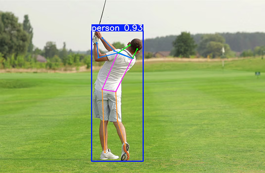
Loading data is a further bottleneck. A single 640 x 640 RGB image at the default input size of Ultralytics YOLO26 holds 1,228,800 values, and amplitude encoding fits them into 21 qubits, but preparing an arbitrary 21-qubit state takes a number of gates that grows with 2²¹, about as many operations as a CPU needs to read the pixels.