Mean average precision (mAP) in object detection
Understand Mean Average Precision (mAP) in Object Detection. Learn its meaning, calculation, and why mAP is key for evaluating model performance.
AI adoption is growing rapidly, and AI is being integrated into various innovations, from self-driving cars to retail systems that can identify products on a shelf. These technologies rely on computer vision, a branch of artificial intelligence (AI) that enables machines to analyze visual data.
A key evaluation metric used to measure the accuracy of computer vision systems and algorithms is mean average precision (mAP). The mAP metric indicates how closely a vision AI model’s prediction matches real-world results.
A common computer vision task is object detection, where a model identifies multiple objects in an image and draws bounding boxes around them. mAP is the standard metric used for evaluating the performance of object detection models and is widely used to benchmark deep learning models like Ultralytics YOLO11.
In this article, we will see how mean average precision is calculated and why it’s essential for anyone training or evaluating object detection models. Let’s get started!
Link to this sectionWhat is mean average precision (mAP)?#
Mean average precision is a score that showcases how accurate a deep learning model is when it comes to tasks related to visual information retrieval, like detecting and identifying different objects in an image. For example, consider an object detection model analyzing a photo that contains a dog, a cat, and a car. A reliable model can perform object detection by recognizing each object and drawing bounding boxes and labels around it, highlighting where it is and what it is.
mAP indicates how well the model performs this task across many images and different types of objects. It checks whether the model accurately identifies each object and its location within the image. The score ranges from 0 to 1, where one means the model found everything perfectly, and zero means it failed to detect any objects.
Link to this sectionKey concepts in mean average precision (mAP)#
Before we explore the concepts behind mean average precision in machine learning, let’s get a better understanding of two basic terms: ground truth and predictions.
Ground truth refers to the accurate reference data, where objects and their locations in the image are carefully labeled by humans through a process known as annotation. Meanwhile, predictions are the results that AI models give after analyzing an image. By comparing the AI model’s predictions to the ground truth, we can measure how close the model came to getting the correct results.
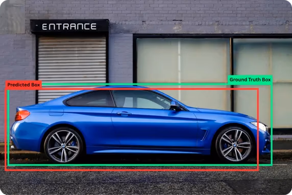
Fig 1. The model prediction and ground truth bounding boxes. Image by author.
Link to this sectionConfusion matrix#
A confusion matrix is often used to understand how precise an object detection model is. It’s a table that shows how the model’s predictions match the actual correct answers (ground truth). From this table, we can get a breakdown of four key components or outcomes: true positives, false positives, false negatives, and true negatives.
Here are what these components represent in the confusion matrix:
- True positive (TP): An object and its location are correctly detected by the model.
- False positive (FP): The model made a detection, but it was incorrect.
- False negative (FN): An object that was actually present in the image, but the model failed to detect it.
- True negative (TN): True negatives occur when the model correctly identifies the absence of an object.
True negatives aren’t commonly used in object detection, since we typically ignore the many empty regions in an image. However, it's essential in other computer vision tasks, such as image classification, where the model assigns a label to the image. For instance, if the task is to detect whether an image contains a cat or not, and the model correctly identifies “no cat” when the image does not contain one, that’s a true negative.
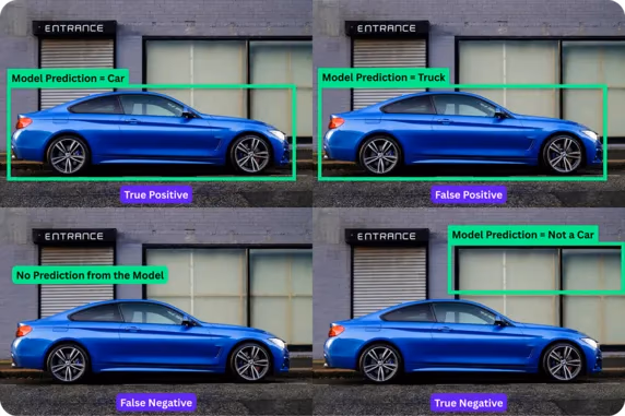
Fig 2. Classification outcomes in a confusion matrix. Image by author.
Link to this sectionIntersection over Union (IoU)#
Another vital metric in evaluating object detection models is Intersection over Union (IoU). For such vision AI models, simply detecting the presence of an object in an image is not enough; it also needs to locate where it is in an image to draw bounding boxes.
The IoU metric measures how closely the model’s predicted box matches the actual, correct box (ground truth). The score is between 0 and 1, where 1 means a perfect match and 0 means no overlap at all.
For example, a higher IoU (like 0.80 or 0.85) means the predicted box is a close match to the ground-truth box, indicating accurate localization. A lower IoU (like 0.30 or 0.25) means the model did not accurately locate the object.
To determine if a detection is successful, we use different thresholds. A common IoU threshold is 0.5, which means a predicted box must overlap with the ground-truth box by at least 50% to be counted as a true positive. Any overlap below this threshold is considered a false positive.
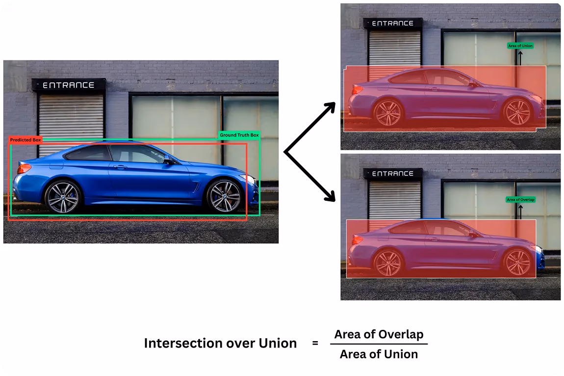
Fig 3. Understanding Intersection over Union. Image by author.
Link to this sectionPrecision and recall#
So far, we’ve explored some basic evaluation metrics for understanding the performance of object detection models. Building on this, two of the most important metrics are precision and recall. They give us a clear picture of how accurate the model’s detections are. Let’s take a look at what they are.
Precision values tell us how many of the model’s predictions were actually correct. It answers the question: of all the objects the model claimed to detect, how many were truly there?
Recall values, on the other hand, measure how well the model finds all the actual objects present in the image. It answers the question: of all the real objects present, how many did the model correctly detect?
Together, precision and recall give us a clearer picture of how well a model is performing. For example, if a model predicts 10 cars in an image and 9 of them are indeed cars, it has a precision of 90% (a positive prediction).
These two evaluation metrics often involve a trade-off: a model can achieve a high precision value by only making predictions it is fully confident in, but this may cause it to miss many objects, which lowers the recall level. Meanwhile, it can also reach very high recall by predicting a bounding box almost everywhere, but this would reduce precision.
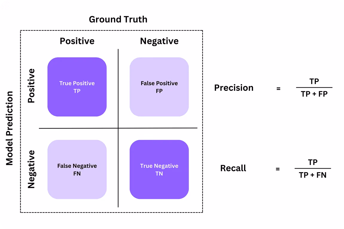
Fig 4. Precision and recall. Image by author.
Link to this sectionAverage precision#
While precision and recall help us understand how a model performs on individual predictions, average precision (AP) can provide a broader view. It illustrates how the model’s precision changes as it attempts to detect more objects, and summarizes its performance into a single number.
To calculate the average precision score, we can first create a combined graph-like metric called a precision-recall curve (or PR curve) for each type of object. This curve shows what happens as the model makes more predictions.
Consider a scenario where the model begins by detecting only the easiest or most obvious objects. At this stage, precision is high because most predictions are correct, but recall is low since many objects are still missed out on. As the model tries to detect more objects, including the harder or rarer ones, it usually introduces more errors. This causes precision to drop while recall increases.
The average precision is the area under the curve (AUC of the PR curve). A bigger area means the model is better at keeping its predictions accurate, even as it detects more objects. AP is calculated separately for each class label.
For example, in a model that can detect cars, bikes, and pedestrians, we can calculate the AP values individually for each of those three categories. This helps us see which objects the model is good at detecting and where it might still need improvement.
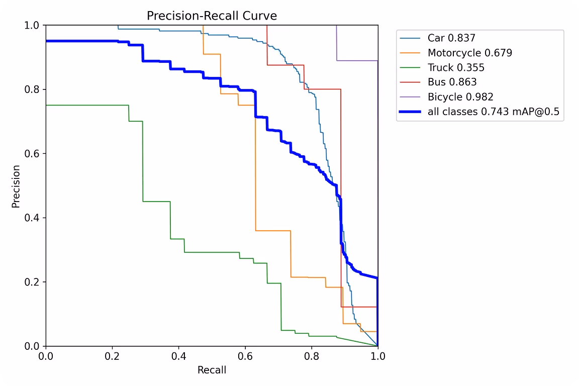
Fig 5. A PR curve for five different classes. (Source)
Link to this sectionMean average precision#
After calculating the average precision for each object class, we still need a single score that reflects the model's overall performance across all classes. This can be achieved using the mean average precision formula. It averages the AP scores for every category.
For instance, let’s assume a computer vision model like YOLO11 achieves an AP of 0.827 for cars, 0.679 for motorcycles, 0.355 for trucks, 0.863 for buses, and 0.982 for bicycles. Using the mAP formula, we can add these numbers and divide by the total number of classes as follows:
mAP = (0.827 + 0.679 + 0.355 + 0.863 + 0.982) ÷ 5 = 0.7432 ≈ 0.743
The mAP score of 0.743 provides a straightforward solution for judging how well the model performs across all object classes. A value close to 1 means the model is accurate for most categories, while a lower value suggests it struggles with some.
Link to this sectionSignificance of AP and mAP in computer vision#
Now that we have a better understanding of how AP and mAP are calculated and what their components are, here’s an overview of their significance in computer vision:
-
Low AP for a specific class: A low AP for a single class often means the model struggles with that specific object class. This can be due to insufficient training data or visual challenges in the images, like occlusion.
-
Localization errors: A higher mAP value at a lower IoU threshold (such as mAP@0.50) combined with a significant drop at a higher IoU threshold (such as mAP@0.75) indicates that the model can detect objects but struggles to localize them precisely.
-
Overfitting: A higher mAP value on the training dataset but a lower mAP value on the validation dataset is a sign of overfitting, making the model unreliable for new images.
Link to this sectionReal-world applications of mean average precision#
Next, let’s explore how key metrics like mAP can help when building real-world computer vision use cases.
Link to this sectionAutonomous vehicles: Why a higher mAP value means safer roads#
When it comes to self-driving cars, object detection is crucial for identifying pedestrians, road signs, cyclists, and lane markings. For instance, if a child suddenly runs across the street, the car has seconds to detect the object (child), locate where it is, track its movement, and take necessary action (apply the brakes).
Models like YOLO11 are designed for real-time object detection in such high-stakes scenarios. In these cases, mAP becomes a critical measure of safety.
A high mAP score ensures the system detects the child quickly, localizes them precisely, and triggers braking with minimal delay. A low mAP can mean missed detections or dangerous misclassifications, such as confusing the child with another small object.
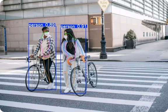
Fig 6. An example of YOLO11 being used to detect pedestrians on the road. (Source)
Link to this sectionUsing mAP for accurate product detection#
Similarly, in retail, object detection models can be used to automate tasks like stock monitoring and checkout processes. When a customer scans a product at a self-checkout, an error in detection can cause frustration.
A high mAP score makes sure the model accurately distinguishes between similar products and draws precise bounding boxes, even when items are tightly packed. A low mAP score can lead to mix-ups. For instance, if the model mistakes an orange juice bottle for a visually similar apple juice bottle, it could result in incorrect billing and inaccurate inventory reports.
Retail systems integrated with models like YOLO11 can detect products in real time, check them against the inventory, and update backend systems instantly. In fast-paced retail settings, mAP plays a crucial role in keeping operations accurate and reliable.
Link to this sectionEnhancing diagnostic accuracy with high mAP in healthcare#
Improving diagnostic accuracy in healthcare starts with precise detection in medical imaging. Models like YOLO11 can help radiologists spot tumors, fractures, or other anomalies from those medical scans. Here, mean average precision is an essential metric for evaluating a model’s clinical reliability.
A high mAP indicates that the model achieves both high recall (identifying the most actual issues) and high precision (avoiding false alarms), which is crucial in clinical decision-making. Also, the IoU threshold in healthcare is often set very high (0.85 or 0.90) to ensure extremely accurate detection.
However, a low mAP score can raise concerns. Let’s say a model misses a tumor; it could delay diagnosis or lead to incorrect treatment.
Link to this sectionPros and cons of using mAP#
Here are the key advantages of using mean average precision to evaluate object detection models:
-
Standardized metric: mAP is the industry standard for evaluating object detection models. A mAP value enables fair and consistent comparisons between different models.
-
Reflects real-world performance: A high mAP indicates that the model excels at detecting various object classes and maintains strong performance in complex, real-world scenarios.
-
Class-wise diagnostics: A mAP score evaluates detection performance for each class individually. This makes it easier to identify underperforming categories (like bicycles or street signs) and fine-tune the model accordingly.
While there are various benefits to using the mAP metric, there are some limitations to consider. Here are a few factors to take into account:
-
Difficult for non-tech stakeholders: Business or clinical teams may find mAP values abstract, unlike more intuitive and easy-to-understand metrics.
-
Doesn’t reflect real-time constraints: mAP doesn’t account for inference speed or latency, which are crucial for deployment in time-sensitive applications.
Link to this sectionKey takeaways#
We have seen that mean average precision is not just a technical score but a reflection of a model's potential real-world performance. Whether in an autonomous vehicle system or a retail checkout, a high mAP score serves as a reliable indicator of a model's performance and practical readiness.
While mAP is an essential and impactful metric, it should be viewed as part of a well-rounded evaluation strategy. For critical applications such as healthcare and autonomous driving, it’s not enough to rely solely on mAP.
Additional factors like inference speed (how quickly the model makes predictions), model size (impacting deployment on edge devices), and qualitative error analysis (understanding the types of mistakes the model makes) must also be considered to ensure the system is safe, efficient, and truly fit for its intended purpose.
Join our growing community and GitHub repository to find out more about computer vision. Explore our solutions pages to learn about applications of computer vision in agriculture and AI in logistics. Check out our licensing options to get started with your own computer vision model today!