Diffusion Models
Explore how diffusion models use generative AI to create high-fidelity data. Learn to enhance Ultralytics YOLO26 training with realistic synthetic data today.
Diffusion models are a class of generative AI algorithms that learn to create new data samples by reversing a gradual noise addition process. Unlike traditional discriminative models used for tasks like object detection or classification, which predict labels from data, diffusion models focus on generating high-fidelity content—most notably images, audio, and video—that closely mimics the statistical properties of real-world data. They have rapidly become the state-of-the-art solution for high-resolution image synthesis, overtaking previous leaders like Generative Adversarial Networks (GANs) due to their training stability and ability to generate diverse outputs.
Link to this sectionHow Diffusion Models Work#
The core mechanism of a diffusion model is based on non-equilibrium thermodynamics. The training process involves two distinct phases: the forward process (diffusion) and the reverse process (denoising).
- Forward Process: This phase systematically destroys the structure of a training image by adding small amounts of Gaussian noise over a series of time steps. As the process continues, the complex data (like a photo of a cat) gradually transforms into pure, unstructured random noise.
- Reverse Process: The goal of the neural network is to learn how to reverse this corruption. Starting from random noise, the model predicts the noise that was added at each step and subtracts it. By iteratively removing noise, the model "denoises" the random signal until a coherent, high-quality image emerges.
This iterative refinement allows for exceptional control over fine details and texture, a significant advantage over single-step generation methods.
Link to this sectionReal-World Applications#
Diffusion models have moved beyond academic research into practical, production-grade tools across various industries.
- Synthetic Data Generation: One of the most valuable applications for computer vision engineers is the creation of synthetic data to augment training datasets. If a dataset lacks diversity—for example, missing images of cars in snowy conditions—a diffusion model can generate realistic variations. This helps improve the robustness of vision models like YOLO26 when deployed in unpredictable environments.
- Image Inpainting and Editing: Diffusion models power advanced editing tools that allow users to modify specific regions of an image. This technique, known as inpainting, can remove unwanted objects or fill in missing parts of a photo based on the surrounding context. Architects and designers use this for rapid prototyping, visualizing changes to products or environments without needing manual 3D rendering.
Link to this sectionDifferentiating Key Terms#
It is helpful to distinguish diffusion models from other generative architectures:
- Diffusion Models vs. GANs: While GANs use two competing networks (a generator and a discriminator) and are known for fast sampling, they often suffer from "mode collapse," where the model produces limited varieties of output. Diffusion models are generally more stable during training and cover the distribution of the data more comprehensively, though they can be slower at inference time.
- Diffusion Models vs. VAEs: Variational Autoencoders (VAEs) compress data into a latent space and then reconstruct it. While VAEs are fast, their generated images can sometimes appear blurry compared to the crisp details produced by diffusion processes.
Link to this sectionPractical Implementation#
While training a diffusion model from scratch requires significant compute, engineers can leverage pre-trained models or integrate them into workflows alongside efficient detectors. For instance, you might use a diffusion model to generate background variations for a dataset and then use the Ultralytics Platform to annotate and train a detection model on that enhanced data.
Below is a conceptual example using torch to simulate a simple forward diffusion step (adding noise), which is the foundation of training these systems.
import torch


def add_noise(image_tensor, noise_level=0.1):
    """Simulates a single step of the forward diffusion process by adding Gaussian noise."""
    # Generate Gaussian noise with the same shape as the input image
    noise = torch.randn_like(image_tensor) * noise_level

    # Add noise to the original image
    noisy_image = image_tensor + noise

    # Clamp values to ensure they remain valid image data (e.g., 0.0 to 1.0)
    return torch.clamp(noisy_image, 0.0, 1.0)


# Create a dummy image tensor (3 channels, 64x64 pixels)
dummy_image = torch.rand(1, 3, 64, 64)
noisy_result = add_noise(dummy_image)

print(f"Original shape: {dummy_image.shape}, Noisy shape: {noisy_result.shape}")
Link to this sectionFuture Directions#
The field is rapidly evolving toward latent diffusion models (LDMs), which operate in a compressed latent space rather than pixel space to reduce computational costs. This efficiency makes it feasible to run powerful generative models on consumer hardware. As research continues, we expect tighter integration between generative inputs and discriminative tasks, such as using diffusion-generated scenarios to validate the safety of autonomous vehicles or improve medical image analysis by simulating rare pathologies.