Support Vector Machine (SVM)
Explore Support Vector Machines (SVM). Learn about optimal hyperplanes, the kernel trick, and how SVMs compare to modern models like Ultralytics YOLO26.
Support Vector Machine (SVM) is a robust and versatile supervised learning algorithm widely used for classification and regression challenges. Unlike many algorithms that simply aim to minimize training errors, an SVM focuses on finding the optimal boundary—called a hyperplane—that best separates data points into distinct classes. The primary objective is to maximize the margin, which is the distance between this decision boundary and the closest data points from each category. By prioritizing the widest possible separation, the model achieves better generalization on new, unseen data, effectively reducing the risk of overfitting compared to simpler methods like standard linear regression.
Link to this sectionCore Mechanisms and Concepts#
To understand how SVMs function, it is helpful to visualize data plotted in a multi-dimensional space where each dimension represents a specific feature. The algorithm navigates this space to discover the most effective separation between groups.
- Optimal Hyperplane: The central goal is to identify a flat plane (or hyperplane in higher dimensions) that divides the input space. In a simple 2D dataset, this appears as a line; in 3D, it becomes a flat surface. The optimal hyperplane is the one that maintains the maximum possible distance from the nearest data points of any class, ensuring a clear distinction.
- Support Vectors: These are the critical data points that lie closest to the decision boundary. They are termed "support vectors" because they effectively support or define the position and orientation of the hyperplane. Modifying or removing other data points often has no impact on the model, but moving a support vector shifts the boundary significantly. This concept is central to the efficiency of SVMs, as detailed in the Scikit-learn SVM guide.
- The Kernel Trick: Real-world data, such as complex natural language processing (NLP) datasets, is rarely linearly separable. SVMs address this limitation using a technique called the "kernel trick," which projects data into a higher-dimensional space where a linear separator can effectively divide the classes. Common kernels include the Radial Basis Function (RBF) and polynomial kernels, allowing the model to capture intricate, non-linear relationships.
Link to this sectionSVM vs. Related Algorithms#
Distinguishing SVMs from other machine learning techniques helps practitioners select the correct tool for their predictive modeling projects.
- Logistic Regression: Both are linear classifiers, but their optimization goals differ significantly. Logistic Regression is probabilistic, maximizing the likelihood of the observed data, whereas SVM is geometric, maximizing the margin between classes. SVMs tend to perform better on well-separated classes, while Logistic Regression offers calibrated probability outputs.
- K-Nearest Neighbors (KNN): KNN is a non-parametric, instance-based learner that classifies a point based on the majority class of its neighbors. In contrast, SVM is a parametric model that learns a global boundary. SVMs generally offer faster inference latency once trained because they do not need to store and search the entire dataset at runtime.
- Decision Trees: A decision tree splits the data space into rectangular regions using hierarchical rules. SVMs can create complex, curved decision boundaries via kernels, which decision trees might struggle to approximate without becoming overly deep and prone to overfitting.
- Modern Deep Learning (e.g., YOLO26): SVMs typically rely on manual feature engineering, where experts select relevant inputs. Advanced models like Ultralytics YOLO26 excel at automatic feature extraction directly from raw images, making them far superior for complex perceptual tasks like real-time object detection and instance segmentation.
Link to this sectionReal-World Applications#
Support Vector Machines remain highly relevant in various industries due to their accuracy and ability to handle high-dimensional data.
- Bioinformatics: SVMs are extensively used for protein structure prediction and gene classification. By analyzing complex biological sequences, researchers can identify patterns related to specific diseases, aiding in early diagnosis and personalized medicine.
- Text Categorization: In the field of text summarization and spam filtering, SVMs excel at managing the high dimensionality of text vectors. They can effectively classify emails as "spam" or "not spam" and categorize news articles by topic with high precision.
Link to this sectionImplementation Example#
While modern computer vision tasks often utilize end-to-end models like Ultralytics YOLO26, SVMs are still powerful for classifying features extracted from these models. For example, one might use a YOLO model to detect objects and extract their features, then train an SVM to classify those specific feature vectors for a specialized task.
Below is a concise example using the popular scikit-learn library to train a simple classifier on synthetic data.
from sklearn import svm
from sklearn.datasets import make_classification
from sklearn.model_selection import train_test_split

# Generate synthetic classification data
X, y = make_classification(n_features=4, random_state=0)
X_train, X_test, y_train, y_test = train_test_split(X, y, random_state=0)

# Initialize and train the Support Vector Classifier
clf = svm.SVC(kernel="linear", C=1.0)
clf.fit(X_train, y_train)

# Display the accuracy on the test set
print(f"Accuracy: {clf.score(X_test, y_test):.2f}")
For teams looking to manage larger datasets or train deep learning models that can replace or augment SVM workflows, the Ultralytics Platform provides tools for seamless data annotation and model deployment. Those interested in the mathematical foundations can refer to the original paper by Cortes and Vapnik (1995), which details the soft-margin optimization that allows SVMs to handle noisy real-world data effectively.