Graph Neural Network (GNN)

A graph neural network (GNN) is a neural network that operates directly on graphs: sets of nodes connected by edges, where nodes and edges can both carry features. Molecules (atoms and bonds), social networks (users and follows), road networks (intersections and road segments), 3D meshes, and the joints of a human skeleton are all graphs. A graph has no fixed grid or order, and its nodes have different numbers of neighbors, so the sliding filters of a convolutional neural network (CNN) and the step-by-step reading of a recurrent neural network (RNN) do not apply directly. GNNs handle this with message passing: each node repeatedly updates its feature vector from those of its neighbors, producing node embeddings that encode both a node's own attributes and its position in the graph.

How Message Passing Works#

A GNN layer updates every node in three steps. Each neighbor sends a message, usually a learned transformation of its features. The node aggregates the incoming messages with a function that ignores their order, such as a sum, mean, or maximum. Then it combines the aggregate with its own features to form its new representation. Because the aggregation ignores order, the result does not depend on how the nodes happen to be numbered. Justin Gilmer and colleagues described many GNNs as instances of this message passing neural network framework in 2017. After the last layer, a task-specific head reads the node embeddings to label nodes, predict missing edges, or classify a whole graph:

Each layer extends a node's view by one hop, so after k layers a node's embedding depends on every node within k edges, its receptive field in the graph. The PyTorch snippet below builds a six-node path graph, applies three graph convolution layers with the normalization from Thomas Kipf and Max Welling's GCN, and uses autograd to list which input nodes affect node 0 after each layer:

import torch
from torch import nn

# A path graph 0-1-2-3-4-5 as an adjacency matrix with self-loops
A = torch.eye(6)
for i in range(5):
    A[i, i + 1] = A[i + 1, i] = 1
deg = A.sum(dim=1)
A_hat = A / torch.sqrt(deg[:, None] * deg[None, :])  # GCN normalization D^-1/2 (A + I) D^-1/2

torch.manual_seed(0)
x = torch.randn(6, 4, requires_grad=True)  # 4 input features per node
layers = [nn.Linear(4, 4) for _ in range(3)]

h = x
for k, layer in enumerate(layers, start=1):
    h = torch.tanh(A_hat @ layer(h))  # each node mixes in its neighbors' transformed features
    grad = torch.autograd.grad(h[0].sum(), x, retain_graph=True)[0]
    print(f"After layer {k}, node 0 depends on nodes {grad.abs().sum(dim=1).nonzero().flatten().tolist()}")

It prints [0, 1], [0, 1, 2], and [0, 1, 2, 3]: node 0's receptive field grows by exactly one hop per layer.

Common GNN Architectures#

• GCN: The graph convolutional network computes H′ = σ(D̃^(−1/2) à D̃^(−1/2) H W), where à is the adjacency matrix with self-loops and D̃ its degree matrix: a degree-weighted average over each node and its neighbors, followed by a weight matrix W shared by all nodes.
• GraphSAGE: Samples a fixed number of neighbors per node and learns the aggregator, so it scales to very large graphs and can embed nodes that appear after training.
• GAT: Graph attention networks weight each neighbor with learned attention scores instead of fixed degree-based weights.
• GIN: The graph isomorphism network sums its neighbors and applies an MLP, which Keyulu Xu and colleagues proved makes it as good at telling graphs apart as the Weisfeiler-Lehman test, the upper limit for standard message passing.
• Graph transformers: Apply self-attention across all nodes and add positional encodings derived from the graph structure. A standard transformer is itself a GNN on a fully connected graph of tokens.

Stacking many layers causes over-smoothing: repeated averaging pulls node embeddings toward each other until they become indistinguishable, which is why many GNNs use only two or three layers, as the original GCN did with two. PyTorch Geometric and the Deep Graph Library (DGL) implement these layers efficiently on sparse edge lists.

Real-World Applications#

• Weather forecasting: Google DeepMind's GraphCast, published in Science in 2023, runs message passing on a multi-scale mesh covering the globe and produces 10-day forecasts at 0.25° resolution in under a minute, outperforming the most accurate operational deterministic systems on 90% of 1,380 verification targets.
• Drug discovery: In 2020, MIT researchers trained a directed message passing network to predict antibacterial activity from molecular graphs and used it to identify halicin, a compound structurally unlike known antibiotics that killed many drug-resistant bacteria in laboratory tests.
• Recommendation systems: Pinterest's PinSage learned pin embeddings from a graph of 3 billion pins and boards and 18 billion edges, trained on 7.5 billion examples.
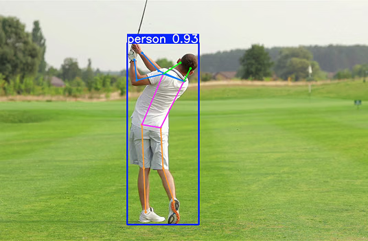
• Skeleton-based action recognition: ST-GCN treats body joints as nodes, connects them by bones within each frame and to the same joint in neighboring frames, and classifies the action from the resulting spatiotemporal graph. YOLO26 pose estimation models return 17 COCO keypoints per person in every frame, the joint coordinates such a skeleton graph is built from.

GNNs vs. Related Concepts#

• Knowledge graph: A data structure that stores facts as entity-relation-entity triples. A GNN is a model that can learn from one, for example to predict missing links.
• Geometric deep learning: The broader field of networks built around the symmetries of their data, covering CNNs on grids, GNNs on graphs, and models on meshes and manifolds.
• CNN: A CNN applied to an image is a special case of message passing on a grid graph. Every pixel there has the same number of neighbors in fixed relative positions, so a CNN can learn a separate weight for each neighbor position, which a GNN on an irregular graph cannot.