Linear Probing
Learn how linear probing evaluates frozen AI representations with logistic regression, feature extraction, and Ultralytics YOLO26 embeddings for transfer learning.
Linear probing is an evaluation and adaptation technique that measures how useful a model’s learned representations are by training a simple linear predictor on top of frozen features. The pretrained encoder remains unchanged, while only a linear layer—often logistic regression for classification—is fitted to labeled data. Strong probe performance suggests that the encoder’s embeddings already organize relevant concepts so they can be separated with simple decision boundaries.
In machine learning, the term is unrelated to linear probing in hash tables, where neighboring storage locations are checked after a collision. In AI and deep learning, it refers specifically to probing a representation with a linear model.
How Linear Probing Works#
A typical neural network contains an encoder or backbone that transforms raw input into a feature vector, followed by a task-specific prediction head. Linear probing follows four steps:
- Pretrain or load an encoder.
- Freeze its parameters so training cannot update them.
- Perform feature extraction on labeled examples.
- Train a linear classifier using those fixed features.
For multiclass classification, the probe is commonly a single dense layer with softmax output or a scikit-learn logistic regression classifier. Although logistic regression includes a nonlinear probability transformation, its class scores and decision boundaries are linear functions of the input features.
Linear probing is especially common in self-supervised learning, where an encoder learns from unlabeled data. The Keras NNCLR example demonstrates this by training a dense classifier over a frozen encoder’s features. Because the probe has limited capacity, it cannot easily compensate for weak representations by learning complex nonlinear transformations.
What Linear Probe Performance Reveals#
A linear probe tests whether information is both present and readily accessible in a representation. If images of cats and dogs form separable groups in embedding space, a linear classifier can distinguish them with few trainable parameters. If the information is encoded through a more complicated arrangement, a nonlinear classifier may succeed even when the linear probe performs poorly.
Probe accuracy should therefore be treated as a diagnostic rather than a complete measure of model quality. It can be affected by:
- The selected encoder layer and embedding dimension.
- Input resolution and preprocessing.
- The amount and balance of labeled training data.
- Regularization applied to the linear model.
- Data leakage between training and evaluation sets.
Use a held-out validation dataset, preferably created with a reproducible, stratified procedure such as scikit-learn’s train-test splitting utility. Beyond accuracy, a classification metrics report can expose classes that the representation does not separate consistently.
Linear Probing vs Related Methods#
Linear probing belongs to the broader family of transfer and representation-evaluation methods, but several distinctions matter:
- Linear probing vs fine-tuning: A probe updates only the linear head. Fine-tuning updates some or all encoder weights, giving the model more flexibility but requiring additional compute and increasing the risk of overfitting. The TensorFlow transfer learning guide describes freezing a base model before optionally unfreezing it for fine-tuning.
- Linear probing vs feature extraction: Feature extraction produces the embeddings; linear probing trains and evaluates a predictor on those embeddings.
- Linear probing vs linear regression: Linear regression predicts continuous values. Classification probes generally predict discrete classes with logistic regression or a softmax layer.
- Linear probing vs nearest-neighbor evaluation: A linear probe learns class boundaries. Nearest-neighbor methods classify samples according to nearby stored embeddings without learning those boundaries. The PyTorch transfer learning tutorial calls the closely related frozen-encoder workflow a fixed feature extractor.
Linear Probing with Ultralytics YOLO#
A pretrained Ultralytics YOLO26 classification model can generate image embeddings through the documented model.embed() API. The following example freezes the encoder implicitly by precomputing features, then fits a linear probe to distinguish CIFAR-10 cats from dogs:
import numpy as np
from sklearn.linear_model import LogisticRegression
from sklearn.metrics import accuracy_score
from sklearn.model_selection import train_test_split
from torchvision.datasets import CIFAR10
from ultralytics import YOLO

dataset = CIFAR10(root="data", train=False, download=True)
samples = [(image, label) for image, label in dataset if label in (3, 5)][:400]
images, labels = zip(*samples, strict=True)

encoder = YOLO("yolo26n-cls.pt")
embeddings = encoder.embed(list(images), verbose=False)
features = np.stack([embedding.cpu().numpy() for embedding in embeddings])

x_train, x_test, y_train, y_test = train_test_split(features, labels, test_size=0.25, random_state=42, stratify=labels)
probe = LogisticRegression(max_iter=1000)
probe.fit(x_train, y_train)

predictions = probe.predict(x_test)
print(accuracy_score(y_test, predictions))
Only the logistic regression model learns from the cat and dog labels; the YOLO26 encoder weights remain fixed. This isolates the usefulness of its visual representation rather than measuring its ability to adapt through end-to-end training.
Real-World Applications and Practical Guidance#
-
Evaluating unlabeled pretraining: A robotics team may pretrain an encoder on large volumes of unlabeled warehouse video, then probe its features using a small labeled dataset of forklifts, workers, and pallets. High probe accuracy indicates that the representation may support downstream image classification or detection with limited annotation.
-
Comparing domain suitability: A medical imaging team can freeze several candidate encoders and train identical linear probes for tissue categories. If one encoder performs substantially better under the same split and preprocessing, its representation is a stronger starting point for later fine-tuning.
For fair comparisons, keep the dataset split, feature layer, preprocessing, classifier, and optimization settings constant. Evaluate both linear probing and full fine-tuning when possible: the probe measures accessible information in fixed features, while fine-tuning measures how effectively the complete model can adapt.