Hidden Markov Model (HMM)
A hidden Markov model (HMM) infers a sequence of hidden states from noisy observations. Its parameters, the Viterbi algorithm, and applications.
A hidden Markov model (HMM) is a probabilistic model of a sequence in which a system moves between states that cannot be observed directly, and each hidden state produces an observation that can. Given a sequence of observations, such as audio frames or DNA letters, an HMM computes how likely each sequence of hidden states is, for example the phonemes behind the audio or the gene regions behind the letters. "Markov" refers to its central assumption: the next state depends only on the current state. Leonard Baum and colleagues developed the theory in the late 1960s, and HMMs went on to power speech recognition for decades. Built entirely from explicit probabilities, they remain a standard tool in time series analysis and bioinformatics, and a classic example of statistical AI.
Components of an HMM#
An HMM with N hidden states is defined by three sets of probabilities:
- Initial probabilities (π): The probability of starting in each hidden state.
- Transition probabilities (A): An N × N matrix whose entry
A[i, j]is the probability of moving from state i to state j in one step, which makes the hidden states a Markov chain. - Emission probabilities (B): The probability of each observation given the current state. Discrete observations use a table, and continuous ones, such as acoustic features, use distributions like Gaussian mixtures.
Two assumptions keep the model tractable: each state depends only on the previous state, and each observation depends only on the current state. Unrolled over time, the model is a chain of hidden states, each emitting one observation:
Three Classic HMM Problems#
Lawrence Rabiner's widely cited 1989 tutorial organized HMM use around three questions. Each has a dynamic programming answer whose cost grows with N² × T for T observations, instead of with the Nᵀ possible state sequences:
- Evaluation: How likely is an observation sequence under a given model? The forward algorithm sums over all hidden paths, which is how a recognizer picks the word model that best explains an utterance.
- Decoding: Which hidden state sequence best explains the observations? The Viterbi algorithm, which Andrew Viterbi published in 1967 for decoding convolutional codes, finds the single most likely path, and the forward-backward algorithm gives the probability of each state at each time step.
- Learning: Which parameters best fit a set of observation sequences? The Baum-Welch algorithm, an instance of expectation maximization, estimates π, A, and B from unlabeled sequences. When the state sequences are labeled, counting transitions and emissions is enough.
Viterbi decoding fits in a few lines of NumPy. In this model a person's activity, walking or running, is hidden, a tracker reports one speed reading per frame, and activities tend to persist from frame to frame:
import numpy as np

states = ["walk", "run"]
start = np.array([0.8, 0.2])  # initial state probabilities
trans = np.array([[0.9, 0.1], [0.1, 0.9]])  # activities tend to persist between frames
emit = np.array([[0.7, 0.25, 0.05], [0.1, 0.3, 0.6]])  # P(speed | state) for slow, medium, fast
obs = [0, 0, 2, 0, 0, 1, 2, 2, 1, 2]  # per-frame speed readings

# Viterbi: best log-probability of reaching each state, plus back-pointers
logp = np.log(start) + np.log(emit[:, obs[0]])
back = []
for o in obs[1:]:
    scores = logp[:, None] + np.log(trans)  # rows: previous state, columns: next state
    back.append(scores.argmax(axis=0))
    logp = scores.max(axis=0) + np.log(emit[:, o])

# Trace the most likely state sequence backward from the best final state
path = [int(logp.argmax())]
for pointers in reversed(back):
    path.insert(0, int(pointers[path[0]]))
print("Speeds: ", " ".join(["slow", "medium", "fast"][o] for o in obs))
print("Decoded:", " ".join(states[s] for s in path))
It decodes walk walk walk walk walk run run run run run. The fast reading at frame 3 stays "walk", because switching to running and back would take two unlikely transitions, and the medium readings at frames 6 and 9 become "run" because of the fast frames around them. A per-frame classifier that ignored transitions would have labeled frame 3 as running.
HMMs vs. Related Models#
- Kalman filter: Runs the same predict-and-update recursion for continuous states with linear dynamics and Gaussian noise. The HMM forward algorithm is its counterpart for discrete states.
- Bayesian networks: An HMM is the simplest dynamic Bayesian network, with one hidden and one observed variable per time step.
- Markov decision process (MDP): Adds actions and rewards to a Markov chain with observed states, the framework behind reinforcement learning.
- Recurrent neural networks and transformers: Learn long-range, nonlinear dependencies from large datasets and have replaced HMMs in most speech and language tasks. HMMs need far less data, and every one of their probabilities can be read directly.
- State space models (SSMs): Deep learning layers such as Mamba share the state-space idea from control theory and update a continuous hidden vector with learned, deterministic dynamics.
Real-World Applications#
- Speech recognition: From the 1980s until the early 2010s, most recognizers modeled each phoneme as a small HMM with Gaussian mixture emissions. Deep neural networks then took over the emission model in hybrid systems, and end-to-end models later replaced the HMM altogether.
- Bioinformatics: Profile HMMs describe families of related protein or DNA sequences. HMMER uses them to search sequence databases for distant relatives and underlies the Pfam protein family database, and gene finders label stretches of a genome as coding or noncoding with HMMs.
- Part-of-speech tagging: Early statistical natural language processing tagged words as nouns, verbs, and other parts of speech by Viterbi decoding over tag sequences.
- Activity recognition: Sequences of body poses or wearable sensor readings decode into activities such as standing, walking, or falling. The Ultralytics workouts monitoring solution tracks a two-state sequence of this kind: it labels each person "up" or "down" from a joint angle in YOLO26 pose estimation keypoints, the elbow by default, switching above 145° and below 90°, and counts a repetition at each up-to-down change.