Hyperspectral Imaging
Hyperspectral imaging records a reflectance spectrum for every pixel across hundreds of narrow bands, identifying materials that look alike in RGB.
Hyperspectral imaging (HSI) records a full spectrum of reflected or emitted light for every pixel of an image, sampled in tens to hundreds of narrow, contiguous wavelength bands. Those narrow bands resolve the absorption features that minerals, plant pigments, plastics, and tissues leave at characteristic wavelengths, so a pixel's spectrum, its spectral signature, identifies what a surface is made of even when two materials look identical to a color camera. The result is a three-dimensional data cube with two spatial axes and one spectral axis, which computer vision and machine learning models read either one pixel spectrum at a time or as a joint spatial-spectral volume. NASA's Jet Propulsion Laboratory has flown its AVIRIS airborne spectrometer since the late 1980s, recording 224 contiguous bands from 400 to 2,500 nanometers.
How a Hyperspectral Camera Builds the Data Cube#
An imaging spectrometer splits incoming light by wavelength with a prism, a diffraction grating, or a set of filters and records it on a two-dimensional detector. Since the detector has only two dimensions, the third axis of the cube comes from scanning:
- Pushbroom (line-scan): A slit admits one line of the scene, the spectrometer spreads that line's light across the detector by wavelength, and the cube builds up line by line as the aircraft, satellite, or conveyor belt moves.
- Whiskbroom: A rotating mirror sweeps a single point across the scene, as in the classic AVIRIS instrument.
- Spectral scanning: A tunable filter captures one full image per band in sequence, which suits microscopes and other static scenes.
- Snapshot: A filter mosaic on the sensor captures the whole cube in a single exposure at video rates, at the cost of spatial resolution.
Hyperspectral vs. Multispectral and RGB Imaging#
An RGB camera records three broad bands, and multispectral imaging records a handful of broad bands chosen in advance, such as the 13 bands of ESA's Sentinel-2 satellites, enough for vegetation indices like NDVI. Hyperspectral sensors sample the spectrum contiguously: NASA's EMIT imaging spectrometer on the International Space Station records 285 bands between 381 and 2,493 nanometers, about 7.5 nanometers apart. That detail costs data volume, a lower signal-to-noise ratio per band, and strong correlation between neighboring bands, so pipelines often compress the cube with principal component analysis or band selection before training, a form of dimensionality reduction. Satellite image analysis uses both kinds of imagery, and sensor fusion often pairs a hyperspectral cube with LiDAR elevation or high-resolution RGB.
Analyzing Hyperspectral Data with AI#
Raw sensor counts are first converted to reflectance with radiometric calibration and, for airborne and satellite data, atmospheric correction, as part of data preprocessing. Classic methods then compare each pixel against reference spectra: the spectral angle mapper scores the angle between two spectra regardless of brightness, and linear unmixing estimates what fraction of a mixed pixel each pure material, or endmember, contributes. Deep learning models classify 1D spectra, run 2D convolutional neural networks on principal components, or apply 3D convolutions and transformers to spatial-spectral patches. Without labels, anomaly detection flags pixels whose spectra differ from the scene's background, such as a gas plume or a camouflaged object.
Pixel classification, the hyperspectral form of semantic segmentation, is benchmarked on small airborne scenes such as Indian Pines, captured by AVIRIS over northwestern Indiana at 145×145 pixels with 224 bands, 200 after removing water-absorption bands, and 16 crop and land-cover classes, and Pavia University, captured by the ROSIS sensor at 610×340 pixels with 103 bands and 9 classes. Random pixel splits from a single scene put neighboring, nearly identical pixels into both training and test sets, a form of data leakage that inflates accuracy, so reliable evaluations hold out spatially separate regions.
Ultralytics YOLO reads the number of input channels from the channels key of a dataset YAML and loads multi-channel TIFF images, so a YOLO26 object detection model can train on a stack of selected bands or principal components, as the 10-channel COCO8-Multispectral dataset demonstrates.
Real-World Applications#
- Precision agriculture: Water stress, nutrient deficiency, and disease alter chlorophyll and water absorption features in leaf spectra, so cameras on drones and aircraft map crop health field by field.
- Recycling and food sorting: Near-infrared line-scan cameras above conveyor belts tell polymers such as PET, polyethylene, and polypropylene apart by their absorption spectra, and food lines use the same principle to find foreign material and bruising.
- Medical image analysis: Oxygenated and deoxygenated hemoglobin absorb light differently, so hyperspectral cameras map tissue oxygen saturation and perfusion for wound assessment and surgery without contrast agents.
- Earth observation: EMIT was built to map the minerals in desert dust sources, and the same shortwave-infrared measurements resolve methane's absorption features, which has let the instrument locate methane plumes from landfills and oil and gas facilities around the world.