Model Predictive Control (MPC)
Learn how model predictive control (MPC) predicts outcomes, optimizes actions within constraints, and works with computer vision in robotics and building control.
Model predictive control (MPC) is a way to choose actions by predicting how a system will respond over the next several moments, selecting the best sequence of actions, and carrying out only the first one. Then it measures what actually happened and plans again. Think of a warehouse robot approaching a turn: rather than steering solely from its current position, it considers where different steering choices would leave it—and whether those paths would clear nearby shelves.
How Does MPC Work?#
An MPC controller needs a state, such as a robot’s position and speed; a dynamics model, which predicts how actions change that state; and an objective, which describes a good outcome. Its optimization might favor reaching a destination while penalizing abrupt steering. Constraints rule out or discourage unacceptable behavior, such as exceeding a motor’s speed limit or entering an occupied space.
At each control interval, MPC predicts the consequences of candidate actions across a prediction horizon. It chooses the sequence with the lowest overall cost, applies its first action, and repeats with updated measurements. This repeated replanning is called receding-horizon control. The MathWorks introduction to MPC illustrates this feedback loop; its guide to sample time and horizons explains why looking farther ahead can improve anticipation but increase computation.
There is no single universal “MPC formula.” In plain language, the controller minimizes the predicted sum of goal-tracking errors and action costs over its horizon, subject to its model and constraints. The do-mpc explanation of MPC also shows how this idea extends to nonlinear systems, whose responses cannot be adequately represented by a simple linear model.
What Do the Model and Measurements Contribute?#
The dynamics model predicts consequences, not necessarily images. It might estimate how a robot’s position changes when wheel speeds change, or how a room’s temperature responds to heating and outdoor weather. Its parameters can come from physical knowledge, measured data, or predictive modeling. Learning the model does not eliminate the need to test whether its predictions remain accurate in the operating environment.
Measurements correct the plan. Cameras may reveal obstacles, but an image detection is not automatically a usable physical position. A controller may need camera calibration, distance information, and a state estimator to combine observations with motion history. A Kalman filter is one possible estimator; the MathWorks guide to controller state estimation explains why MPC often estimates states it cannot measure directly. Replanning helps with imperfect forecasts, but it cannot make a delayed or unreliable observation safe by itself.
Where Is MPC Applied?#
- Warehouse robot navigation: A mobile robot uses camera observations and its own motion estimates to plan a short path around workers and shelving. An MPC controller can compare steering and speed sequences against a travel-time goal and motion limits, then revise its choice as people move. The Nav2 predictive controller documentation provides a practical robotics example of evaluating predicted trajectories.
- Building climate control: A building controller can predict how heating or cooling decisions will affect room temperatures over the coming hours. Occupancy estimates and weather forecasts help it prepare for demand while balancing energy use and comfort limits. The US Department of Energy’s building sensors and controls overview describes this combination of machine learning and predictive control.
In both cases, the benefit is not prediction alone. MPC uses predictions to choose an action within operational limits, then checks its plan against the next observation.
How Is MPC Different from Related Concepts?#
A world model represents how an environment may evolve; MPC is a control procedure that uses a dynamics model to compare possible actions. Reinforcement learning typically learns how to act from experience, whereas MPC explicitly solves a forward-looking planning problem during operation. They can be combined: a learned model may supply MPC’s predictions.
Likewise, object tracking estimates where an object is across frames; it does not choose steering commands. Tracking can supply observations to MPC, but the controller still needs a motion model, objective, constraints, and an optimization method. The MathWorks constraint guide distinguishes hard limits from soft constraints that permit a penalized violation.
How Can Computer Vision Support an MPC Pipeline?#
Ultralytics YOLO26 can provide a perception input through object detection. This documented inference workflow returns bounding boxes for one image:
from ultralytics import YOLO

# Load a pretrained detection model.
model = YOLO("yolo26n.pt")

# Observe objects in the current image.
results = model("https://ultralytics.com/images/bus.jpg")
result = results[0]

# Inspect image-space locations available to a perception pipeline.
print(result.boxes.xyxy)
The output gives box coordinates in image space—not distances, velocities, or control commands. For a moving scene, YOLO tracking mode can help maintain object identities, while depth estimation can provide distance estimates. A separate estimation and MPC system must turn suitable observations into a state, predict action outcomes, solve the constrained optimization, and command the hardware.
Before deployment, test that the full perception-to-action loop finishes within its control interval. Evaluate missed detections, model mismatch, and cases where constraints make a plan infeasible; set a defined fallback behavior rather than assuming the optimizer will always return a safe command.