Epipolar Geometry
Epipolar geometry relates two views of a scene, confining each point's match to a line in the other image, the basis of stereo depth and 3D mapping.
In computer vision, epipolar geometry describes the geometric relationship between two camera views of the same scene. A pixel in one image corresponds to a ray of possible 3D points, and that ray projects into the second image as a line, the epipolar line, on which the pixel's match must lie. The constraint depends only on the cameras' internal parameters and relative pose, independent of the scene's structure, and it turns the search for a match from the whole image into a search along one line. That makes epipolar geometry the foundation of stereo vision, structure from motion, and the visual SLAM that guides robots and headsets. Richard Hartley and Andrew Zisserman's Multiple View Geometry in Computer Vision is the standard reference.
Epipoles, Epipolar Lines, and the Epipolar Plane#
The two camera centers and any scene point define a plane, the epipolar plane. The line joining the camera centers is the baseline, and it pierces each image plane at the epipole, the image of the other camera's center, which may lie outside the frame or at infinity. Each epipolar plane cuts each image in an epipolar line, also called an epiline, so all epipolar lines in an image pass through its epipole. As the scene point slides along the first camera's viewing ray, its projection in the second image slides along the epipolar line.
Fundamental and Essential Matrices#
The fundamental matrix F, a 3 × 3 matrix of rank two, captures the whole relationship in pixel coordinates. For corresponding points x and x′ written in homogeneous form (x, y, 1), the epipolar constraint is x′ᵀ F x = 0, and the product F x gives the coefficients of x's epipolar line in the second image. When the cameras are calibrated through camera calibration, the essential matrix E = K′ᵀ F K expresses the same constraint in normalized coordinates and factors into the relative rotation R and translation t as E = [t]ₓ R. Christopher Longuet-Higgins introduced the essential matrix and the eight-point algorithm in 1981, and Olivier Faugeras, Quang-Tuan Luong, and Richard Hartley developed the uncalibrated fundamental matrix in the early 1990s. Because E fixes only the direction of t, two views alone give the scene's shape up to an unknown scale, and a known baseline or object size sets the scale.
Both matrices are estimated from matched keypoints, such as SIFT features, with a robust estimator such as RANSAC that repeatedly fits the matrix to a minimal sample of matches and keeps the model most matches agree with. This example builds two views of 100 points, replaces 20 matches with random wrong ones, and estimates F with OpenCV's MAGSAC variant of RANSAC:
import cv2
import numpy as np

rng = np.random.default_rng(0)
K = np.array([[800.0, 0, 320], [0, 800.0, 240], [0, 0, 1]])  # intrinsics shared by both cameras

# 100 scene points seen by two cameras; the second sits 0.5 m to the right, turned 5 degrees
points = rng.uniform([-2, -1, 4], [2, 1, 8], (100, 3))
rvec = np.array([0.0, np.radians(5), 0.0])
tvec = -cv2.Rodrigues(rvec)[0] @ np.array([0.5, 0.0, 0.0])
x1 = cv2.projectPoints(points, np.zeros(3), np.zeros(3), K, None)[0].reshape(-1, 2) + rng.normal(0, 0.5, (100, 2))
x2 = cv2.projectPoints(points, rvec, tvec, K, None)[0].reshape(-1, 2) + rng.normal(0, 0.5, (100, 2))
x2[:20] = rng.uniform([0, 0], [640, 480], (20, 2))  # replace 20 matches with wrong ones

# Robust estimation keeps the matches that agree with a single fundamental matrix
F, inliers = cv2.findFundamentalMat(x1, x2, cv2.USAC_MAGSAC, 1.0)
kept = inliers.ravel() == 1
print(f"Kept {kept[20:].sum()} of 80 true matches and {kept[:20].sum()} of 20 wrong ones")

# Each point in image 1 defines a line a*x + b*y + c = 0 in image 2 that its match must lie on
lines = cv2.computeCorrespondEpilines(x1, 1, F).reshape(-1, 3)
dist = np.abs((lines[:, :2] * x2).sum(axis=1) + lines[:, 2])
print(f"Median distance to epipolar line: {np.median(dist[20:]):.2f} px (true), {np.median(dist[:20]):.0f} px (wrong)")
print(f"Wrong match that survived: {dist[:20][kept[:20]].round(2)} px from its line")
It keeps 75 of the 80 true matches and rejects 19 of the 20 wrong ones. True matches lie a median 0.43 pixels from their epipolar lines, set by the half-pixel noise, and wrong ones 144 pixels. The one wrong match that survives happens to land 0.61 pixels from its line, since the constraint confines a match to a line and only appearance can pick the right point along it.
A pure rotation has no baseline, and a single plane fits many fundamental matrices equally well, so both cases are handled with a homography, the 3 × 3 mapping between views of a plane. ORB-SLAM initializes its map by fitting a homography and a fundamental matrix in parallel and keeping the one that explains the matches better.
Rectification, Disparity, and Depth#
Rectification warps a stereo pair so that its epipolar lines become horizontal and aligned, placing every match on the same image row. Stereo matchers then search each row, and the column offset between matches, the disparity d, gives depth Z = f × B / d for focal length f and baseline B, which is how stereo rigs produce depth estimation maps. The KITTI stereo benchmark scores such matchers on rectified scenes from autonomous driving.
Applications Beyond Stereo#
In 3D reconstruction, COLMAP verifies every image pair by fitting fundamental, essential, or homography matrices and discards pairs and matches without enough geometric support. Image matching pipelines use the same check to reject false correspondences, and image registration takes the homography branch above when the scene is flat or the camera only rotates, as in panorama stitching. Between two frames of a moving camera, the epipolar constraint holds only for static surfaces, so optical flow vectors that violate it reveal independently moving objects. Multi-camera capture of human pose associates the same person across views by how close their joints fall to each other's epipolar lines before triangulating a 3D skeleton, with an Ultralytics YOLO26 pose estimation model supplying 17 COCO body keypoints per person in each view.